
![]()
| Brightline Ridership and Revenue Study |
|
| Phase I Study: Southeast Florida and Orlando Phase II Study: Extension to Tampa |
|
| September 2018 |
![]()
Disclaimer
This Report was prepared by The Louis Berger U.S., Inc., (LB) for the benefit of All Aboard Florida Operations, LLC (Client) pursuant to a Professional Services Agreement dated May 17, 2017.
LB has performed its services to the level customary for competent and prudent engineers performing such services at the time and place where the services to our Client were provided. LB makes or intends no other warranty, express or implied.
Certain assumptions regarding future trends and forecasts may not materialize, which may affect actual future performance and market demand, so actual results are uncertain and may vary significantly from the projections developed as part of this assignment. The data used in the Report was current as of the date of the Report and may not now represent current conditions.
The Report is provided for information purposes only. LB makes no representations or warranty that the information in the Report is sufficient to provide all the information, evaluations, and analyses necessary to satisfy the entire due diligence needs of a reader of this report.
| 1 | P a g e |
Table of Contents
| Executive Summary | 7 | |||||
| ES-1 | Overview of the Investment Grade Study Process | 8 | ||||
| ES-2 | Study Process | 9 | ||||
| ES-3 | Overview of the Brightline Rail Service | 10 | ||||
| ES-4 | Relevant Market for High Speed Rail | 11 | ||||
| ES-5 | Key Assumptions | 13 | ||||
| ES-6 | Key Findings and Ridership and Revenue Forecast | 15 | ||||
| 1.0 |
Introduction |
19 | ||||
| 1.1 |
Organization of Report |
20 | ||||
| 2.0 |
Travel Market Socioeconomic and Demographic Conditions |
21 | ||||
| 2.1 |
Population |
22 | ||||
| 2.2 |
Population Forecasts |
24 | ||||
| 2.3 |
Employment |
28 | ||||
| 2.4 |
Employment Forecasts |
30 | ||||
| 2.5 |
Income |
31 | ||||
| 2.6 |
Travel and Tourism |
32 | ||||
| 2.7 |
Domestic Visitation |
34 | ||||
| 2.8 |
International Visitation |
34 | ||||
| 3.0 |
Intercity Travel Market for Brightline |
36 | ||||
| 3.1 |
Addressable Market Geography for Brightline |
37 | ||||
| 3.2 |
Travel Market for Brightline Phase I Study |
38 | ||||
| 3.2.1 | Bus | 38 | ||||
| 3.2.2 | Long-Distance Rail (Amtrak) | 41 | ||||
| 3.2.3 | Short-Distance Rail (Tri-Rail) | 42 | ||||
| 3.2.4 | Air | 45 | ||||
| 3.2.5 | Auto | 47 | ||||
| 3.3 |
Travel Market for Brightline Phase II Study |
54 | ||||
| 3.3.1 | Bus | 54 | ||||
| 3.3.2 | Rail (Amtrak) | 56 | ||||
| 3.3.3 | Air | 57 | ||||
| 3.3.4 | Auto | 59 | ||||
| 3.3.5 | Airport Access Trips | 64 | ||||
| 4.0 |
Brightline Travel Demand Model |
66 | ||||
| 4.1 |
Overview of Methods |
66 | ||||
| 2 | P a g e |
| 4.2 |
Survey Design |
66 | ||||
| 4.2.1 | Screening | 66 | ||||
| 4.2.2 | Reference Trip | 67 | ||||
| 4.2.3 | Choice Exercise | 67 | ||||
| 4.2.4 | Induced Travel | 69 | ||||
| 4.2.5 | Socioeconomic Characteristics | 69 | ||||
| 4.3 |
Survey Implementation and Summary |
69 | ||||
| 4.3.1 | Survey Implementation and Summary for Brightline Phase I Study | 69 | ||||
| 4.3.2 | Survey Implementation and Summary for Brightline Phase II Study | 72 | ||||
| 4.4 |
Mode Choice Model Estimation |
75 | ||||
| 4.4.1 | Conceptual Overview | 75 | ||||
| 4.4.2 | Summary of Model Estimation Process (Phase I Study) | 77 | ||||
| 4.4.3 | Summary of Model Estimation Process (Phase II Study) | 80 | ||||
| 4.5 |
Travel Demand Model Development |
80 | ||||
| 4.5.1 | Level of Service Assumptions | 81 | ||||
| 4.5.2 | Model Calibration | 91 | ||||
| 4.5.3 | Induced Ridership | 92 | ||||
| 5.0 |
Brightline Ridership and Revenue Forecast |
94 | ||||
| 5.1 |
Overall Level of Ridership and Revenue |
94 | ||||
| 5.1.1 | Ramp-Up | 96 | ||||
| 5.1.2 | Methodological Overview | 96 | ||||
| 5.2 |
Fare Revenue Estimation |
97 | ||||
| 5.3 |
Network Model Ridership & Revenue Forecasts |
98 | ||||
| 5.3.1 | Market Capture and Compatibility with Existing Modes of Travel | 98 | ||||
| 5.4 |
Overall Forecast Summary |
103 | ||||
| 5.4.1 | Forecast Growth Comparison | 103 | ||||
| 5.5 |
Segment Loading and Boardings & Alightings |
103 | ||||
| 5.6 |
Phase II Study Lakeland Station Impacts |
105 | ||||
| 6.0 |
Forecast Sensitivity |
106 | ||||
| 6.1 |
Brightline Travel Time |
106 | ||||
| 6.2 |
Brightline Frequency |
106 | ||||
| 6.3 |
Intercity Travel Time by Auto |
107 | ||||
| 6.4 |
Auto Fuel Prices |
107 | ||||
| 6.5 |
Air Fares |
107 | ||||
| 7.0 |
Conclusion |
108 | ||||
| 3 | P a g e |
| Appendix A Population Density | 109 |
| Appendix B Employment Density | 114 |
| List of Figures and Tables | |
| Figure ES-1 The Study Area of Phase I and Phase II of the Study | 7 |
| Figure ES-2 Brightline Annual Ridership Forecast, 2018-2040 | 16 |
| Figure ES-3 Brightline Fare Revenue Forecast, 2018-2040 (2016 $) | 17 |
| Figure ES-4 Brightline Long-Distance Market Share, 2023 | 17 |
| Figure ES-5 Brightline Short-Distance Market Share, 2023 | 18 |
| Figure 1-1 Proposed Route and Stations | 19 |
| Figure 2-1 Study Area | 21 |
| Figure 2-2 Study Area Population Density | 22 |
| Figure 2-3 POPULATION, 1975-2015 (IN THOUSANDS) | 23 |
| Figure 2-4 COMPOUND ANNUAL GROWTH RATE IN POPULATION | 24 |
| Figure 2-5 MPO POPULATION FORECAST BY COUNTY, 2010-2040 (IN THOUSANDS) | 25 |
| Figure 2-6 SOUTHEAST FLORIDA POPULATION FORECAST | 26 |
| Figure 2-7 CENTRAL FLORIDA POPULATION FORECAST | 26 |
| Figure 2-8 LAKELAND POPULATION FORECAST | 27 |
| Figure 2-9 LAKELAND POPULATION FORECAST | 27 |
| Figure 2-10 Study Area Employment Density | 28 |
| Figure 2-11 Employment 1975-2015 (in Thousands) | 29 |
| Figure 2-12 Employment Forecasts by Region 2010-2040 (Thousands) | 30 |
| Figure 2-13 REAL PER CAPITA PERSONAL INCOME, 1975-2015 (2017 DOLLARS) | 31 |
| Figure 2-14 HISTORICAL TRENDS IN FLORIDA VISITATION: 2006-2015 | 32 |
| Figure 2-15 TRAVEL RELATED EMPLOYMENT IN FLORIDA | 33 |
| Figure 2-16 ANNUAL VISITATION BY THEME PARK | 33 |
| Figure 3-1 Travel Time to Nearest Brightline Station | 37 |
| Figure 3-2 Market Catchment Areas | 38 |
| Figure 3-3 Historical Growth in Intercity Bus Travel in the United States | 40 |
| Figure 3-4 Amtrak Florida Station Boardings | 41 |
| Figure 3-5 Tri-Rail System Map | 43 |
| Figure 3-6 Tri-Rail System Ridership | 44 |
| Figure 3-7 Annual Air Traffic Volume between Central and Southeast Florida | 45 |
| Figure 3-8 Comparison of Air Traffic Volumes | 46 |
| Figure 3-9 Florida Turnpike Central-to-Southeast Florida Historical Traffic Counts | 48 |
| Figure 3-10 I-95 Central-to-Southeast Florida Historical Traffic Counts | 48 |
| Figure 3-11 Southeast Florida Historical Traffic Counts | 50 |
| Figure 3-12 Southeast Florida Historical Traffic Counts | 50 |
| Figure 3-13 Florida Turnpike Traffic Model Performance (Actual Vs. Fitted – Monthly) | 53 |
| Figure 3-14 Econometric Analysis and Projection of Florida Turnpike Traffic (Monthly) | 53 |
| Table 3-13 Estimated Daily Intercity Long-Distance Bus Person Trips | 54 |
| Figure 3-15 Ridership Benchmark From RSG | 55 |
| Table 3-14 Projected Daily Intercity Bus Person Trips | 55 |
| Figure 3-16 Amtrak Florida Station Boardings (Thousands) | 56 |
| Table 3-15 Historical and Future Amtrak Passenger Volumes | 56 |
| 4 | P a g e |
| Figure 3-17 Annual Air Traffic Volume between Tampa and Southeast Florida | 57 |
| Table 3-16 Annual Air Passenger Volumes, FAA 10% Ticket Sample | 57 |
| Figure 3-18 FAA’s Terminal Area Forecasts For Airport Enplanements In Study Area | 58 |
| Figure 3-19 Passenger Volume Share Of Enplanement In Origin And Destination Airport | 59 |
| Figure 3-20 Prediction Of Future Passenger Volume Between City Pairs | 59 |
| Figure 3-21 Counter stations identified for historical traffic volume | 61 |
| Figure 3-22 Historical AADT Trend At Counter Stations | 62 |
| Table 3-17 Summary Of Historical Aadt And Cagr | 62 |
| Table 3-18 Estimated Daily Auto Person Trips By Time Of Day | 63 |
| Table 3-19 Annual Auto Person Trips Projection | 64 |
| Table 3-20 Current And Future Airport Access Choice Trips By Mode | 65 |
| Figure 4-1 Example Stated Choice Exercise | 68 |
| Figure 4-2 LONG DISTANCE MODE CHOICE MODEL NESTED LOGIT STRUCTURE | 77 |
| Figure 4-3 SHORT DISTANCE MODE CHOICE MODEL NESTED LOGIT STRUCTURE | 79 |
| Figure 5-1 Brightline Annual Ridership Forecast – Base Case | 95 |
| Figure 5-2 Brightline Annual Revenue Forecast – Base Case | 95 |
| Figure 5-3 Comparison of Brightline Fares to Amtrak Northeast Corridor Fare Rates | 98 |
| Figure 5-4 Long-Distance Travel Network Model Market Shares, 2023 | 99 |
| Figure 5-5 Share of Brightline Ridership by Source (Long-Distance) | 100 |
| Figure 5-6 Brightline Ridership Market Draw by Source (Long-Distance) | 100 |
| Figure 5-7 Share of Brightline Ridership by Source (Short-Distance), 2023 | 101 |
| Figure 5-8 Share of Brightline Ridership by Source (Short-Distance) | 102 |
| Figure 5-9 Brightline Ridership Market Draw by Source (Short-Distance) | 102 |
| Figure 5-10 Comparison of Brightline Forecast Growth Rates | 103 |
| Table ES-1 Brightline Ridership and Revenue Forecast, 2023 (2016 $) | 16 |
| Table ES-2 Sensitivity Test Results, Ridership and Revenue % Change, 2023 | 18 |
| Table 3-1 Estimated Daily Intercity Long-Distance Bus Person Trips | 39 |
| Table 3-2 Estimated Daily Short-Distance Bus Person Trips | 39 |
| Table 3-3 Projected Daily Intercity Long-Distance Bus Person Trips | 40 |
| Table 3-4 Projected Daily Short-Distance Bus Person Trips | 40 |
| Table 3-5 Historical and Future Amtrak Passenger Volumes | 42 |
| Table 3-6 Current and Projected Daily Short-Distance Rail Trips | 44 |
| Table 3-7 Annual Air Passenger Volumes, FAA 10% Ticket Sample | 46 |
| Table 3-8 Estimates of Air Passengers in the Brightline Service Travel Market | 47 |
| Table 3-9 Estimated Daily Long-Distance Auto Person Trips | 51 |
| Table 3-10 Estimated Daily Short-Distance Auto Person Trips | 51 |
| Table 3-11 Long-Distance City Pair O-D Shares | 52 |
| Table 3-12 Short-Distance City Pair O-D Shares | 52 |
| Table 5-1 2023 Ridership & Revenue | 94 |
| Table 5-2 Ramp-up Comparisons | 96 |
| Table 5-3 Average Fares (Smart Class), 2016 $ | 97 |
| Table 5-4 Average Fares (Select Class), 2016 $ | 97 |
| Table 5-5 Long-Distance Travel Network Model Market Shares by City Pair, 2023 | 99 |
| Table 5-6 Short-Distance Travel Network Model Market Shares by City Pair, 2023 | 101 |
| Table 5-7 Forecast Brightline – Annual Segment Volumes and Revenues (2016 $) | 104 |
| Table 5-8 Brightline Daily Boardings and Alightings, 2023 | 104 |
| 5 | P a g e |
| Table 5-9 Brightline Daily Boardings and Alightings, 2030 | 105 |
| Table 5-10 Lakeland Station Ridership and Revenue Impacts | 105 |
| Table 6-1 Sensitivity Test Results, Ridership and Revenue % Change, 2023 | 106 |
| 6 | P a g e |
Executive Summary
All Aboard Florida Operations, LLC commissioned Louis Berger U.S., Inc. (LB) to develop an investment grade ridership and revenue forecast study for the re-introduction of passenger rail service on its existing right of way. The proposed new passenger rail service, named Brightline, will be a privately owned and operated, intercity service connecting key cities in Southeast Florida with key cities in Central Florida and Tampa Area. This study was conducted in two distinct phases, the Phase I Study evaluated Brightline service between Southeast Florida and Orlando as indicated in Figure ES-1, while the Phase II Study evaluated the incremental ridership and revenue associated with an extension of service to Tampa with an intermediate stop at Disney World.
The objective of this study is to provide an independent overview of ridership and revenue that will inform and advance the project planning efforts and decisions of potential investors and funding partners.
| 7 | P a g e |
ES-1 Overview of the Investment Grade Study Process
The ridership and fare revenue forecasts presented in this report are characterized as being investment-grade in that they provide a level of information in data gathering and analysis that is typical of that required to support investment decision-making.1 The comprehensive nature of this study is underpinned by the following key features:
| ● | Independent approach by experienced travel demand forecasting consultants. |
| ● | Forecasting models constructed from the bottom up using data gathered from regional planning agencies, stakeholder organizations, and recognized commercial sources. |
| ● | Stated Preference Survey designed to measure characteristics of existing intercity travel demand. |
| ● | Pricing Research survey data to support findings on willingness to pay and induced demand |
| ● | A critical, benchmarked assessment of economic growth projections that are used to estimate the overall future growth in travel demand. |
| ● | The development of a forecasting models for Brightline based on current travel, transport system and economic growth data. |
| ● | Alternative model estimates (sensitivity testing) intended to quantify the impacts of different assumptions of key forecasting inputs on forecast results. |
| ● | Emphasis on near term forecasts—investment decision makers commonly place greater emphasis on the early years of operation than the later years (which include growth that is expected, but not certain, to occur). |
Outputs of the forecast that were used to determine the economic, financial, and business planning dimensions of the proposed investment include the following:
| ● | Overall ridership demand estimates |
| ● | Station-station segment ridership estimates |
| ● | Market share analysis |
| ● | Market breakdown by user type (business/non-business, etc.) and geography |
| ● | Ridership demand with respect to level of service |
| ● | User benefit metrics (values-of-time) |
Louis Berger segmented its technical approach and analysis into five distinct areas of study outlined below. Each of these study areas are discussed in greater detail within their respective chapters of this report.
| ● | Market assessment (Section 2, 3) |
| ● | Travel demand model development and calibration (Section 4) |
| ● | Ridership and revenue forecast (Section 5) |
| ● | Sensitivity testing (Section 6) |
1 The key features noted in this section are intended to produce reasonable and reliable forecast estimates. However, it is not possible to forecast future events with certainty. Assumptions regarding economic growth, competition between modes, and external factors affecting overall travel demand and Brightline usage may prove inaccurate. Changes from these assumptions could produce lower or higher ridership than the estimates contained in this report. Please see our disclaimer for more information.
| 8 | P a g e |
ES-2 Study Process
To determine the extent and magnitude of the demand for a new mode of travel between Central Florida, Tampa Area and Southeast Florida, Louis Berger undertook a thorough assessment of the existing and potential future intercity travel market, the attributes of the current modes of travel in the corridor, and prospects for future growth. The study included the following key activities.
| ● | Research to Establish Market Size and Catchment Area– Residents and visitors to cities in the corridor make hundreds of millions of trips per year, but only a select portion of these trips involve travel between the central business districts and surrounding activity centers that would be served by Brightline stations. To identify the addressable market, Louis Berger gathered extensive data on current levels of travel between the city pairs by mode, trip purpose, and time (time of day, day of week). Louis Berger used vendor-provided mobile phone data and findings from recent primary research on traveler preferences to determine the size of the market. The research established an addressable market of over 413 million intercity trips per year in areas reasonably served by the stations (see Section 3). These findings on the size and characteristics of the market are consistent with previous studies undertaken for rail projects in Florida, and provide a conservative base for the demand forecast. |
| ● | Identification of Travel Network and Competing Modes of Travel – The demand forecasting process also requires a thorough understanding of the travel network and the schedule, journey time, and cost attributes of all modes of travel using the network. This report outlines the assumptions and data sources Louis Berger used to establish the highway, rail, and air travel network. The report also documents the attributes of each mode of travel used as inputs to the demand forecast (see Section 4). |
| ● | Assessment of the Prospect for Growth in Travel – An investment grade forecast requires thorough examination of the prospect for growth in the overall travel market. By gathering data from regional transportation planning agencies and other accepted public and commercial sources, Louis Berger established conservative and reasonable growth rates for the overall market based on observed trends in each segment. Based on observed trends in each of the metropolitan regions within the corridor, Louis Berger expects the overall number of long-distance intercity trips between Central and Southeast Florida to grow by 2.9 percent per year; and between Tampa Area and Southeast Florida to grow by 2.2 percent per year. Louis Berger expects the overall number of shorter-distance trips between the cities in Southeast Florida to grow by 1.2 percent per year and between Central Florida and Tampa Area to grow by 2.2 percent per year (see Section 3). |
| ● | Primary Research on Traveler Preferences and Willingness to Pay – When travelers choose to make a journey by auto or by rail they weigh the time and money cost of travel and make a choice based in part on their travel budget and willingness to pay. Travel behavior is also influenced by trip purpose (e.g., business, leisure, commute, airport access) and other factors such as party size and need for a vehicle at the destination. The Brightline system is an entirely new type of service for the region whose unique features can only be tested in hypothetical scenarios that place Brightline against other competing modes. The current state-of-the-practice uses mode choice Stated Preference survey (SP) as the basis for understanding how individuals (or groups of individuals) value individual attributes, such as access time, in-vehicle travel time, headways, and cost - of a transportation choice (see Section 4 for description of the survey, administration, and analysis). Louis Berger also reviewed findings from a recent Pricing |
| 9 | P a g e |
Research survey conducted by Integrated Insights to benchmark data on traveler trip purpose, travel frequency, and willingness to pay (see Section 5).
| ● | Demand Forecasting – The Louis Berger study team employed best practices in discrete choice analysis and network travel demand forecasting to determine diversions from existing modes of travel to Brightline and ridership volumes on the Brightline system by city-pair segment. SP survey responses were used to develop a statistical model of mode choice and estimates of the passenger rail market share and is the basis of the Brightline ridership forecast (see Section 4). |
| ● | Sensitivity Testing– The report provides the findings of sensitivity tests demonstrating the effect of changes in key forecast assumptions on ridership and revenue (see Section 6). These sensitivity tests are used to establish the stability of the forecast model and inform project planning. |
This study was carried out in the context of previous public and private sector sponsored rail implementation studies in Florida that attempted to better understand the potential of passenger rail to relieve congestion and promote mobility and economic development. Louis Berger evaluated the following studies and used them as benchmarking references for the findings in this analysis:
| ● | Florida Overland Express (FOX): Public-private partnership between FDOT and FOX for high speed rail connecting Tampa, Orlando, and Miami. The State withdrew support for the project, in 1999. |
| ● | Investment Grade Ridership Study for the Tampa-Orlando corridor: Performed in 2002 on behalf of the Florida High Speed Rail Authority. The Florida High Speed Rail Enterprise published a two-page update to that forecast in September 2009. |
| ● | In 2006, FDOT prepared the Florida Intercity Passenger Rail Vision Plan, a plan that builds upon previous studies exploring the potential of high speed rail to assist in meeting the State’s mobility needs. |
ES-3 Overview of the Brightline Rail Service
The Phase I of proposed Brightline service will provide new express passenger rail service connecting Orlando with three key urban areas in Southeast Florida – West Palm Beach, Fort Lauderdale, and Miami. The Phase II of proposed Brightline service will provide expanded service beyond Orlando to Lakeland and Tampa Area, with additional stops at Disney World and Meadow Woods. The Brightline service will be privately owned and operated by All Aboard Florida Operations, LLC and will primarily run along the existing transportation corridors including a rail corridor currently used for freight rail operations by Florida East Coast Railway, and an existing highway corridor being accessed in partnership with the State of Florida and other regional governmental entities. Brightline services are unique for Florida: no intercity rail alternative comparable to the proposed Brightline service exists currently. Special features include the following:
| ● | Travel time savings: Substantial time savings to current users of auto, bus, traditional rail and even air traveling between the city pairs |
| ● | Frequency: Consistent, hourly departures seven days per week to fit the schedules of both business and leisure travelers |
| ● | Booking: Online and mobile booking with reserved coach and business class seating for easy boarding |
| ● | Amenities: Free Wi-Fi, convenient outlets, comfortable seating, food and beverage service and related amenities on board |
| 10 | P a g e |
| ● | Stations: Modern, centrally located stations in Southeast Florida and Tampa Area cities, and an airport-based station in Orlando, with good intermodal connectivity (i.e. connections to Metrorail, Metromover, Tri-Rail – with direct connection to Miami International Airport – Broward County Transit, The WAVE Streetcar, and SunRail), parking and ridesharing services available |
In addition to the travel time savings offered by Brightline, the ease of travel and related amenities to the service described above are expected to draw a substantial amount of travelers who attribute a high value to comfort, productivity, and efficiency.
ES-4 Relevant Market for High Speed Rail
With a population of 6.01 million in 2015, the South Florida metropolitan area is the most populous metropolitan area in the Southeastern United States and the fourth most populous urbanized area in the United States. Main cities include Miami, Fort Lauderdale, Pompano Beach, West Palm Beach, and Boca Raton. Miami International Airport is the busiest airport in Florida (38.6 million passengers in 2015) and ranks second in the United States in terms of international passenger count, with 21.2 million international passengers annually. Central Florida’s main city, Orlando, and the surrounding Greater Orlando region attracted 68 million visitors in 2016. Attractions include Walt Disney World Resort, Universal Orlando Resort and SeaWorld Parks & Entertainment. Convention and trade show attendance at the Orange County Convention Center, in 2015 equaled 1.4 million. In addition, a record 22.6 million people visited Tampa Bay Area; Orlando and Miami are among top three visitor sources, leading a high demand for travelling between Central Florida and Tampa Area and between Southeast Florida and Tampa.
Orlando International Airport, a station location, is the second busiest airport in Florida after Miami International Airport with 41.9 million passengers in 2016. Orlando’s secondary airport, Orlando Sanford International Airport had 2.75 million passengers in 2016 while cruise traffic at Port Canaveral accounted for 3.9 million passengers. A total of 18.7 percent of overseas non-resident travelers enter the United States through one of the main South Florida and Central Florida airports: Miami International Airport (12.4 percent); Orlando International Airport (4.1 percent) and Fort Lauderdale International Airport (2.2 percent).
Auto vehicles are the dominant mode of intercity travel between Orlando and the Southeast Florida cities that Brightline will serve. The two main routes between the cities are the I-95 and the Florida Turnpike. Free-flow driving times between Miami and Orlando are estimated at approximately 4 hour 15 minutes along the I-95 and at 3 hour 50 minutes along the Florida Turnpike, which is a toll road. Travel times during congested peak periods can be substantially greater. Air, rail and bus account for a small proportion of trips between the Orlando and Miami; most passengers traveling by air on the more than thirty daily flights between Miami and Orlando are connecting to another destination. Two AMTRAK trains, the Silver Meteor and the Silver Star, each run once daily between Orlando and Southeast Florida. The Silver Meteor, which is the fastest because it does not make a detour to Tampa, takes about 3 hour 45 minutes from Orlando to West Palm Beach and 5 hours 35 minutes from Orlando to Miami. In addition, there are a few private bus companies that operate several buses daily between Orlando and Southeast Florida along the Florida Turnpike. Similarly, auto vehicles play a major role in intercity travel between Tampa Area and the Southeast Florida cities. The major route connecting these two areas is I-75, via which the free-flow driving time is
| 11 | P a g e |
estimated at approximately 4 hours. Air, rail and bus together only account for 10 percent of total trips between these two areas.
Travel between Central Florida and Tampa Area is almost exclusively by auto, accounting for 99 percent of total trips. The main alternative mode of travel is bus: private bus companies provide several daily commuting bus service connecting Orlando and Tampa, with travel time up to 70 minutes. Travel within Southeast Florida is also mostly by automobile. Between Miami and West Palm Beach the Florida Turnpike runs parallel with I-95. Driving from Miami to West Palm Beach takes about 1 hour 17 minutes on the I-95 and 1 hour 27 minutes on the Turnpike. Driving time between Miami and Fort Lauderdale is about 35 minutes while the drive from Fort Lauderdale to West Palm Beach takes about 50 minutes. During congested peak periods it is not uncommon for these travel times to increase by 30 to 50 percent due to incidents or weather making journey and arrival times during these key periods unreliable. The main alternative mode of transportation is rail. Tri Rail, a commuter rail line run by the South Florida Regional Transportation Authority (SFRTA) links Miami, Fort Lauderdale, and West Palm Beach. The 71-mile line has 18 stops and an annual ridership of 4.2 million.
According to the 2016 INRIX Global Traffic Scorecard, the Central and South Florida highways are the most congested in the State, which results in millions of hours of travel delay and excessive fuel consumption and pollutant emissions. Southeast Florida is ranked as the 10th most congested urban area globally in terms of peak hours spent in congestion and has the 5th worst traffic congestion in the United States2. State and local agencies have been active in evaluating alternatives to the severe congestion on north-south roadway links. In June 2010, FDOT prepared the I-95 Transportation Alternatives Study, in consultation with the Department of Law Enforcement, the Department of Environmental Protection, the Division of Emergency Management, the Office of Tourism, Trade and Economic Development and affected MPOs and regional planning councils located along the corridor. The study, which provides an assessment of concerns and proposed solutions related to I-95, found that “I-95 is overwhelmed with traffic demand” and that “[t]ravel within specific urban areas along the I-95 corridor is highly congested in peak travel periods due to single driver automobile use.” This study concluded, among other things, that “[p]assenger rail service presents a mobility option to serve Florida’s East Coast along the I-95 corridor” with multiple benefits including the reduction of “fossil fuel use and greenhouse gases (GHGs); job creation and economic development around station locations; and, better connectivity between northern and southern sections of Florida.”
The potential for intercity rail as a viable alternative has long been recognized by many, including FDOT, which developed the Florida Intercity Passenger Rail “Vision Plan” (FDOT, August 2006). Among other things, the plan found that the state’s intercity travel market would grow at an average annual rate of 3.5% from 2006 to 2040 (FDOT, August 2006). This increase will exacerbate existing transportation problems and require significant development of new infrastructure to meet the needs of this market. In June 2009, FDOT released the 2009 Florida Rail System Plan: Policy Element (FDOT, March 2009), which updated the 2006 Florida Freight and Passenger Rail Plan and built upon previous rail planning efforts, including the 2006 Florida Intercity Passenger Rail Vision Plan to show that:
| ● | There is a rising public interest in rail options to meet intercity and regional mobility needs; |
2http://inrix.com/press-releases/los-angeles-tops-inrix-global-congestion-ranking/
| 12 | P a g e |
| ● | The existing congestion on Florida’s highways may be mitigated by a passenger rail alternative, which would also serve to increase the mobility of tourists, business travelers, and citizens – especially older Floridians; and |
| ● | Reliance on alternate transit options is expected to increase in light of growing concerns over dependence on foreign oil, fluctuating gas prices, and fuel supply disruptions as a result of natural disasters. |
ES-5 Key Assumptions
In order to provide the level of information appropriate for evaluation by lenders and investors during the planning stage of project development, Louis Berger made several key assumptions for the Base Case Forecast, as follows:
| ● | The forecast study area is limited to the extent of the metropolitan areas in Central and Southeast Florida and Tampa Area. Station market catchment areas and trip filters were developed to establish reasonable boundaries for the addressable market and to eliminate illogical station access patterns. As described in Section 3, this is the basis for establishing the size of the candidate market at over 31 million trips per year for the long-distance journey between Orlando and the three cities in Southeast Florida and between Tampa Area and Southeast Florida. When trips between the three cities in Southeast Florida and trips between Tampa Area and Central Florida are considered along with long distance trips, the number grows to over 413 million. |
| ● | Base year trip tables used in the model were developed separately for each mode available between each city pair. As noted in Section 3.6, Louis Berger relied on mobile phone location data purchased from a third-party vendor to determine origin-destination patterns and the size of the automobile trip travel market, which is predominant in size within the addressable market geography. This data was calibrated to volumes on the Florida Turnpike and other intercity routes and verified through an econometric model that linked economic variables to traffic growth on the Florida Turnpike and other intercity routes (that basis of the data being a traffic station counter representative of the Central-Southeast Florida traffic). The data was further adjusted downward to capture captive auto users and lower visitation volumes. Trips tables for other modes of travel were based on information obtained from relevant planning agencies and operators. |
| ● | Brightline fares assumed in the modeling process were provided by All Aboard Florida Operations, LLC and validated by Louis Berger, as outlined in Section 5.2. All fares and competing mode costs were fixed in real terms. For purposes of estimating the future cost of auto travel, gas prices were set at future levels estimated by the U.S. Energy Information Administration (EIA) reference case forecasts referenced in Section 4.5. This report assumes that over the long term, motor fuel will remain in adequate supply and future increases in fuel price will align with the current outlook of these EIA forecasts. In addition, future changes in fares for Brightline, made during the course of operations or otherwise, that differ from those outlined in this Report, may result in levels of ridership and/or revenue that differ from the forecast estimates contained in this Report. Costs associated with competing modes of intercity travel or modes access/egress to Brightline stations different from those assumed in this Report may result in levels of ridership and/or revenue that differ from the forecast estimates contained in this Report. |
| 13 | P a g e |
| ● | The estimation of the future travel market does not include any changes in the location of households or employment related to transit-oriented development in the areas surrounding the stations. |
| ● | We assume that the trajectory of growth in trips will align with the information and estimates presented in Section 3. |
| ● | Congested auto travel times were accounted for in estimating station access and long-distance auto travel times, as summarized in Section 4.5. Given the history of growth in highway congestion and challenges in expanding the highway network, regional planners consider it likely that congestion within and between the regions will increase, making non-highway modes of travel more competitive. Changes in highway capacity or capacity or service levels associated with competing modes of intercity travel or modes access/egress to Brightline stations different from those assumed in this Report may result in levels of ridership and/or revenue that differ from the forecast estimates contained in this Report. |
| ● | Brightline presents users with a premium service unlike any other service in the State of Florida. It is often the case that Stated Preference surveys which underlie the mode choice model and forecast do not fully capture the value that users attribute to the premium nature of services such as Brightline. Our survey research and fare price benchmarking was designed to compensate for this providing the basis for a comprehensive view on traveler willingness to pay. |
| ● | Induced demand potential was based on a method of evaluating the improvement in the generalized cost of travel that has been accepted in other studies for high speed transportation in the U.S. As a novel form of transportation in Florida, Brightline is likely to experience ridership demand for tourism and leisure travel based on its convenience and amenities. |
| ● | This report assumes no major recession or significant economic restructuring will occur which could substantially reduce trip-making and traffic in the region. |
| ● | This report assumes no natural disasters will occur that could significantly alter travel patterns throughout the area served by Brightline. |
| ● | This report assumes no local, regional, or national emergency will arise which would abnormally restrict Brightline service, use of Brightline stations or connectivity to stations, or the use of motor vehicles, or other modes of travel, for station access and egress. |
Any significant departure from these basic assumptions could materially affect estimated Brightline ridership and revenue. Assumptions regarding economic growth, competition between modes and external factors affecting overall travel demand and Brightline usage are subject to uncertainty and may prove inaccurate. As noted herein, Louis Berger has relied on information developed by third parties regarding travel patterns and the outlook for economic conditions. Changes from these assumptions could produce lower or higher ridership than the estimates contained in this report. Please see our disclaimer for more information.
| 14 | P a g e |
ES-6 Key Findings and Ridership and Revenue Forecast
Our forecast evaluation revealed that introduction of Brightline service would complement existing modes of travel and draw a substantial number of business and non-business travelers. Station locations offered by Brightline in Miami, Ft. Lauderdale, West Palm Beach, Orlando (International Airport & Disney), and Tampa will provide an alternative source of transportation for travelers with origins or destinations at or near these urban cores. The thorough study effort resulted in the following key findings:
| ● | Substantial “Addressable Market” – Hundreds of millions of trips are taken annually between the four cities that will be served by Brightline. Louis Berger’s study included a determination of the portion of these total trips that both originate and terminate within a defined distance of a proposed Brightline station (a station “catchment area”). The Brightline addressable market is assumed to include only those trips beginning and ending within station catchment areas, as further defined in 2.10 of this report. Based upon detailed analysis, Louis Berger concluded that the addressable market for Brightline intercity service amounts to over 413 million trips made by individuals annually. |
| ● | Demonstrated Market Travel Growth – Intercity travel on the Florida Turnpike between Orlando and Miami grew by an average of 3.2 percent per year from 2001 to 2016. Average annual growth on I-95 from 2001 to 2015 was approximately 2.1 percent. |
| ● | Demonstrated Market Demographic Growth – In the past 30 years, population in the market area has grown by an annual average of 2.5 percent and employment has grown by an annual average of 3 percent. Within one mile of proposed Brightline stations, annual population growth has ranged from 2 percent to 5 percent since 1990 indicating strong growth in the urban core at the heart of the Brightline alignment. |
| ● | No Comparable Service – Brightline can provide travel time savings of 25% to 50% when compared to existing surface modes (auto, bus and rail) and with a journey time of around three hours from Orlando to Miami is competitive with air on door-to-door travel times. There is no comparable service to Brightline for intercity travel in the existing market. |
| ● | Established Willingness to Pay – The fares used in this study are backed up by two primary research efforts – a Stated Preference Survey and a Pricing Research Study commissioned by the project sponsor – which confirmed willingness to pay for the Brightline service at the price points utilized. Fares are highly competitive with existing modes of travel when time, tolls, and travel costs are considered and are comparable to other successful rail services in the U.S. |
| ● | Long-Standing Interest – Given the profile of the travel market and the central location of the rail line, there has been interest among stakeholders and the public in developing passenger service on the Florida East Coast corridor for decades. |
Estimated Ridership
Louis Berger prepared estimates for annual ridership and farebox revenue for both the short- and long-distance markets of the Brightline service. This forecast accounts for all elements important to future ridership potential including targeted market segments and induced ridership. Table ES-1 summarizes ridership and revenue for 2023, the first year stabilized ridership for the entire system is achieved.
| 15 | P a g e |
Table ES-1 Brightline Ridership and Revenue Forecast, 2023 (2016 $)
| Phase I Study (Miami-Orlando) | Phase II Study (Extension to Tampa) | Grand Total | |||||
| Short-Distance | Long-Distance | Subtotal | Short-Distance | Long-Distance | Subtotal | ||
| Ridership | 3,079,472 | 3,534,197 | 6,613,669 | 1,967,353 | 935,992 | 2,903,345 | 9,517,014 |
| Fare Revenue | $100,763,367 | $298,773,216 | $399,536,583 | $34,053,816 | $145,891,900 | $179,945,716 | $579,482,299 |
| (1) | Short-distance (Phase I Study): Miami-Ft. Lauderdale, Miami-West Palm Beach (WBP), Ft. Lauderdale – WPB |
| (2) | Long-distance (Phase I Study): Southeast Florida-Orlando |
| (3) | Short-distance (Phase II Study): Disney-Orlando Airport, Tampa-Orlando |
| (4) | Long-distance (Phase II Study): Southeast Florida -Tampa |
Ridership and revenue for the initial years of Brightline is expected to start at relatively low levels and grow to a stabilized volume after two years for each segment of operations that is introduced. The low initial levels represent the time it takes for ridership to build up to long-term forecast levels as travelers become acquainted with the new rail service and adjust their trip-making habits. During 2017, management has made substantial investment in marketing, pre-launch ticket sales, and corporate block sales prior to the commencement of full-scale revenue service between Miami and West Palm Beach in May 2018. Management also intends to implement reduced price fares during an introductory period following the beginning of revenue service for each segment (see discussion in Section 5.2). Given these plans, for the short-distance trips, Louis Berger assumed, therefore, 40 percent of forecasted volumes in 2018, and 80 percent forecasted volumes in 2019. For the long-distance trips, Louis Berger assumed a two calendar year ramp-up period: ridership volumes for 2021 are 40 percent of forecasted volumes and 80 percent of forecasted volumes in 2022. These ramp-up assumptions are appropriate to estimation of initial year ridership and revenue, and are consistent with previous rail service forecasts in Florida (see discussion in Section 5.1.1 – Ramp-Up). The forecasts include the assumption that long-distance revenue service will begin in first quarter of 2021. The full service will reach stabilized volumes by 2023. Ridership and revenue for the full forecast length is summarized in the two figures below. The values for 2018-2023 account for ramp-up reductions.
Figure ES-2 Brightline Annual Ridership Forecast, 2018-2040
![]()
Source: Louis Berger, 2017, 2018
| 16 | P a g e |
Figure ES-3 Brightline Fare Revenue Forecast, 2018-2040 (2016 $)
![]()
Source: Louis Berger, 2018, 2018
Estimated Market Share
The forecast indicates that after the initial ramp up period, Brightline will serve approximately 10 percent of the overall market for travel between Southeast Florida and Orlando and approximately 15 percent of the market between Southeast Florida and Tampa. In the short-distance market, Brightline will serve approximately 0.74 percent of the overall market in Southeast Florida, and approximately 11 percent of the market between Tampa and Orlando (this includes the Disney to Orlando Airport travel market).
Figure ES-4 Brightline Long-Distance Market Share, 2023
![]()
Source: Louis Berger, 2017, 2018
| 17 | P a g e |
Figure ES-5 Brightline Short-Distance Market Share, 2023
![]()
Source: Louis Berger, 2017, 2018
Louis Berger conducted a series of sensitivity tests to evaluate the impact that changes in key input variables have on the ridership and revenue forecast. Table ES-2 presents the key assumptions that were altered and the corresponding impact on ridership and revenues for both the short- and long-distance market.
Table ES-2 Sensitivity Test Results, Ridership and Revenue % Change, 2023
| Sensitivity Test Assumption Modified | Change in Assumption | Phase I Study | Phase II Study | ||||||
| Short-Distance | Long-Distance | Short-Distance | Long-Distance | ||||||
| Ridership Effect | Revenue Effect | Ridership Effect | Revenue Effect | Ridership Effect | Revenue Effect | Ridership Effect | Revenue Effect | ||
| Brightline Travel Time | 10% decrease | 3.60% | 4.00% | 6.30% | 6.30% | 2.93% | 3.75% | 6.96% | 7.06% |
| 10% increase | -3.50% | -3.80% | -5.90% | -6.00% | -3.47% | -4.40% | -7.97% | -8.08% | |
| Brightline Frequency | 20% decrease | -3.70% | -3.90% | -1.50% | -1.60% | -6.26% | -5.41% | -1.82% | -1.83% |
| 20% increase | 3.80% | 4.00% | 1.50% | 1.60% | 3.89% | 3.36% | 1.11% | 1.11% | |
| Intercity Travel Time by Auto | 20% decrease | -10.40% | -10.90% | -11.20% | -11.40% | -10.95% | -13.01% | -11.95% | -11.86% |
| 20% increase | 11.90% | 12.60% | 12.60% | 12.70% | 12.19% | 14.99% | 13.28% | 13.16% | |
| Auto Fuel Prices* | Low: (-35% /-31%) | -3.30% | -3.50% | -3.10% | -3.10% | -1.72% | -2.90% | -2.29% | -2.30% |
| High: (+79% /+48%) | 7.90% | 8.40% | 7.40% | 7.50% | 2.81% | 4.75% | 3.67% | 3.68% | |
| Air Fares | 20% decrease | N/A | N/A | -0.30% | -0.30% | N/A | N/A | -1.94% | -2.12% |
| 20% increase | N/A | N/A | 0.10% | 0.10% | N/A | N/A | 1.67% | 1.85% | |
Source: Louis Berger, 2017, 2018
| 18 | P a g e |
| 1.0 | Introduction |
Each year, travelers make hundreds of millions of trips between the communities in Southeast and Central Florida and Tampa Area, making the region one of the most actively traveled areas in the United States. All Aboard Florida Operations, LLC initially commissioned Louis Berger U.S., Inc. (LB) to develop an investment grade ridership and revenue forecast study for the re-introduction of passenger rail service named Brightline.
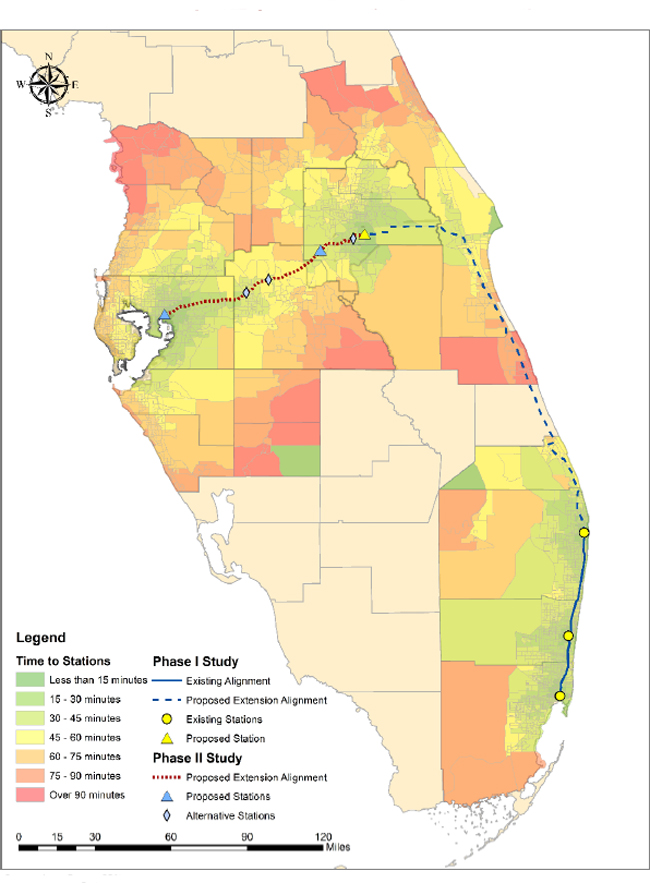
An initial evaluation (hereafter referred to as the Phase I study) evaluated potential Brightline ridership demand associated with an alignment that connected through Miami, Fort Lauderdale and West Palm Beach in Southeast Florida, continued north along an existing rail right-of-way before turning west linking to the Orlando International Airport as shown in Figure 1-1. The initial Phase I Study investment grade analysis effort was conducted using a customized travel demand model based in part on Stated Preference survey research data collected in both Central and Southeast Florida in 2012 and was completed in December of 2017.
Brightline commenced passenger rail operations in Southeast Florida in January of 2018 and plans are currently underway to extend service to Orlando with a connection at the Intermodal facility at Orlando International Airport.
Figure 1-1 Proposed Route and Stations
![]()
Following the completion of the Phase I Study and the commencement revenue passenger service, Louis Berger was once again commissioned to evaluate the incremental ridership potential of extending service to Tampa with an intermediate stop at Disney World and the consideration of some potential alternative station locations along the
| 19 | P a g e |
Interstate 4 (I-4) corridor as also indicated in Figure 1-1.This follow up study (hereafter referred to as the Phase II Study) was conducted using a separate travel demand model based on primary market research data collected in 2018 that focused on both the Tampa-Orlando and Tampa/Lakeland-Southeast Florida travel corridors.
| 1.1 | Organization of Report |
Due to the differences in the travel demand models and the time frames of both the Phase I and Phase II Studies, this report presents elements of the analysis with appropriate distinctions of the two efforts. Furthermore, Louis Berger views the estimated Phase II Study ridership and revenue demand as incremental to the Phase I Study estimates.
| 20 | P a g e |
| 2.0 | Travel Market Socioeconomic and Demographic Conditions |
Despite the distances between city centers, the communities and economies of Southeast Florida, Central Florida, Lakeland and Tampa are interconnected in many ways. Substantial numbers of people travel between these areas for work, business, recreation, and other purposes. This section of the report describes the underlying socioeconomic and demographic characteristics of the region as they pertain to the overall intercity travel market and an evaluation of prospects for growth. Figure 2-1 presents the travel market study area that is segmented into four regions:
| ● | Southeast Florida |
| ● | Central Florida (Orlando area) |
| ● | Lakeland (Polk County) |
| ● | Tampa |
Figure 2-1 Study Area
![]()
Source: Louis Berger. 2018
| 21 | P a g e |
| 2.1 | Population |
The study area consists of three major metropolitan regions with a total population of 11 million in 2017. Over 6 million people live in Southeast Florida, making it the seventh ranked urbanized area in the nation (behind New York, Los Angeles, Chicago, Dallas, Houston and Washington) and the most populous metropolitan area in the Southeastern U.S. The Tampa Area counted 2.7 million residents in 2017 and is the third ranked urbanized area in the Southeastern U.S. The Central Florida region counted 2.1 million residents in 2017, making it the fourth most populous metropolitan area in the Southeastern U.S. The Figure 2-2 presents the overview of population density in the study area. Figures of population density at a more granular level are included in Appendix A
Figure 2-2 Study Area Population Density
![]()
Source: Louis Berger, 2018
| 22 | P a g e |
The Central region experienced an average of 2.0 percent growth per year in the 2005-2015 period, 0.9 percent and 1 percent higher than the population growth rate of Southeast Florida and Tampa Area over the same period, respectively (Table 2-1).
Figure 2-3 POPULATION, 1975-2015 (IN THOUSANDS)
![]()
Source: Louis Berger, 2018 from data provided by Woods & Poole Economics, 2017
Table 2–1 Compound Annual Growth Rate in Population
|
Region/County/Area
|
1975-
2015 |
1995-
2015 |
2005-
2015 |
2010-
2015 |
|
Southeast Florida
|
1.9%
|
1.4%
|
1.1%
|
1.5%
|
|
West Palm Beach
|
2.0%
|
1.4%
|
0.8%
|
1.6%
|
|
Broward
|
1.5%
|
1.3%
|
1.2%
|
1.4%
|
|
Miami-Dade
|
2.8%
|
1.7%
|
1.1%
|
1.4%
|
|
Central Florida
|
3.1%
|
2.5%
|
2.0%
|
2.3%
|
|
Orange
|
2.8%
|
2.5%
|
2.0%
|
2.3%
|
|
Osceola
|
5.4%
|
4.3%
|
3.6%
|
3.7%
|
|
Seminole
|
3.0%
|
1.5%
|
1.0%
|
1.2%
|
|
Lakeland Area (Polk County)
|
2.1%
|
1.9%
|
1.7%
|
1.5%
|
|
Tampa Area
|
1.5%
|
1.2%
|
1.0%
|
1.3%
|
|
Hillsborough
|
2.1%
|
2.0%
|
1.7%
|
1.8%
|
|
Pinellas
|
0.9%
|
0.3%
|
0.2%
|
0.7%
|
|
Total Study Area
|
2.0%
|
1.6%
|
1.3%
|
1.6%
|
Source: Louis Berger, 2017 from data provided by Woods & Poole Economics, 2017
| 23 | P a g e |
Figure 2-4 COMPOUND ANNUAL GROWTH RATE IN POPULATION
![]()
Source: Louis Berger, 2018
Population growth in the study area as a whole has had an average annual gain of 2.0 percent since 1975 (see Table 2-1). In the past 20 years the growth rate has moderated to 1.6 percent.
| 2.2 | Population Forecasts |
In Southeast Florida, three MPO regularly update their long-range transportation plans for the three county urbanized areas. These plans include updates to the outlook on the socioeconomic factors that underpin travel demand. These plans include official forecasts for population through 2040 from a base year of 2010. In Central Florida, MetroPlan Orlando is the MPO for Orange County, Osceola County, and Seminole County. The MPO’s 2040 Long Range Transportation Plan includes population projections for 2040. Similarly, Polk County TPO provides population projections for 2040 for the county (Lakeland Area in this report); Hillsborough MPO along with Forward Pinellas (Pinellas’s MPO) and Sarasota/Manatee’s MPO provides population projections for 2040 for Tampa area. Figure 2-5 shows the levels and rates of growth expected by study areas.
| 24 | P a g e |
Figure 2-5 MPO POPULATION FORECAST BY COUNTY, 2010-2040 (IN THOUSANDS)
![]()
Source: Louis Berger, 2018 from MPOs’ 2040 Long Range Transportation Plan. Central Florida is composed of Orange, Osceola, and Seminole counties. Southeast Florida is composed of Palm Beach, Broward, Miami-Dade Counties; Lakeland Area is composed of Polk County; Tampa Area is composed of Hillsborough, Pinellas and Manatee Counties.
The Southeast Florida forecast calls for the region to experience more moderate levels of increase than in the past, growing at an average annual rate of 0.8 percent from the 2010 Census population count. Regional population is expected to reach 7.0 million in 2040, with over 3.3 million residents in Miami-Dade. The Central Florida MPO forecasts growth at an annual average rate of 1.4 percent from the 2010 Census Population count, reaching 2.8 million residents in the MPO by 2040. The Lakeland area MPO (Polk County MPO) forecasts growth at an annual average rate of 1.8 percent from the 2010 Census Population count, reaching 0.9 million residents in the area by 2040; The Tampa area MPOs forecast growth at an annual average rate of 0.9 percent from the 2010 Census Population count, reaching 2.8 million residents in the area by 2040.
In accounting for future growth in intercity trips, Louis Berger utilized the established travel demand forecasts of the MPOs. To ensure that these forecasts represent reasonable levels of growth when compared to more recent projections, Louis Berger undertook a review of alternative population forecast sources.
Two alternative sources were available at the county level. The Bureau of Economic and Business Research (BEBR) at the University of Florida produces population projections based on forecasts of natural increase and net migration flows. These projections are updated annually and include three different levels-low, medium and high.
Louis Berger also obtained projections developed by Woods & Poole Economics, Inc., a private consulting firm that maintains and annually updates county-level projections for the U.S. (CEDDS - Complete Economic and Demographic Data Source, 2017). With its detail and frequent updates, this source is often used for comparison with official estimates in demand forecasts and due diligence studies.
| 25 | P a g e |
Figure 2-6 SOUTHEAST FLORIDA POPULATION FORECAST
![]()
Source: Louis Berger, 2018
Figure 2-7 CENTRAL FLORIDA POPULATION FORECAST
![]()
Source: Louis Berger, 2018
| 26 | P a g e |
Figure 2-8 LAKELAND POPULATION FORECAST
![]()
Source: Louis Berger, 2018
Figure 2-9 LAKELAND POPULATION FORECAST
![]()
Source: Louis Berger, 2018
For the whole study area, BEBR “Low” case is projecting the slowest rate of growth for the region overall; The overall population level in 2040 projected by BEBR “Medium” is 6 percent higher than the MPO forecast. It is important to note that the MPO forecasts for all study areas between the “low” and “medium” case projections provided by BEBR. Woods and Poole see higher prospects for growth for the region in general than the BEBR “Low” and “Medium” case and the MPO forecasts but lower than the BEBR “high” case projection as shown in the Figure 2-6, 2-7, 2-8, and 2-9.
| 27 | P a g e |
| 2.3 | Employment |
The study area contains more than two-third of all employment in the state of Florida. The Southeast Florida region in particular is a major employment center in Florida, comprising one third of the state’s total employment base. Over 6.9 million people worked in the study area in 2015. Figure 2-10 depicts the employment density of study area. Figures of employment density at a more granular level were included in the Appendix B.
Figure 2-10 Study Area Employment Density
![]()
Source: Louis Berger, 2018
| 28 | P a g e |
There was a slight dip in employment between 2005 and 2010 due to the recession and credit crisis; however, employment levels appear to have recovered. The Southeast Florida region has experienced substantial growth since 1975 when it had 1.27 million jobs. Employment in Central Florida totaled almost 1.4 million in 2015, up from 278,000 jobs in 1975. Employment in Tampa area totaled more than 1.4 million in 2015, up from 519,000 jobs in 1975 (Figure 2-11).
Source: Louis Berger, 2018 from data provided by Woods & Poole Economics, 2017
| Region/County/Area | 1975- | 1995- | 2005- | 2010- |
| 2015 | 2015 | 2015 | 2015 | |
| Southeast Florida | 2.7% | 2.3% | 1.6% | 3.4% |
| Palm Beach | 3.7% | 2.7% | 1.3% | 3.6% |
| Broward | 3.2% | 2.2% | 1.3% | 3.1% |
| Miami-Dade | 2.1% | 2.1% | 1.9% | 3.5% |
| Central Florida | 4.1% | 2.9% | 1.8% | 3.6% |
| Orange | 3.8% | 2.7% | 1.9% | 3.7% |
| Osceola | 5.7% | 4.2% | 2.7% | 4.5% |
| Seminole | 4.8% | 2.8% | 0.8% | 2.6% |
| Lakeland Area (Polk County) | 2.0% | 1.6% | 0.5% | 1.9% |
| Tampa Area | 2.6% | 1.6% | 0.5% | 2.5% |
| Hillsborough | 2.9% | 2.0% | 0.9% | 3.1% |
| Pinellas | 2.2% | 1.0% | -0.1% | 1.7% |
| Total Study Area | 2.9% | 2.2% | 1.3% | 3.2% |
| Source: Louis Berger, 2018 from data provided by Woods & Poole Economics, 2017 |
| 29 | P a g e |
Employment growth in the region as a whole has averaged an annual gain of 2.9 percent since 1975 (see Table 2-3). In the past 20 years the growth rate has moderated to 2.2 percent. With the effects of a major recession still being felt, growth since 2005 has averaged 1.3 percent.
| 2.4 | Employment Forecasts |
In Southeast Florida, regional employment is expected to reach 5.4 million in 2040. In Central Florida, employment is expected to grow at 2.1 percent annually, reaching 2.1 million jobs in 2040. In Tampa area, employment is expected to grow at 1.4 percent annually, reaching 2 million jobs (Figure 2-12).
Source: Louis Berger, 2017 from data provided by Woods & Poole Economics, 2017
To ensure that these forecasts represent reasonable levels of growth when compared to more recent projections, Louis Berger undertook a review of alternative employment forecast sources other than Woods & Poole.
The other source involved employment projections was developed by MPOs’ Long Range Transportation Plan. These forecast include projections for 2040. MPO forecasts see higher prospects for growth for the region in general
| 30 | P a g e |
| 2010 | 2040 | CAGR | ||||
| County | MPO | Woods&Poole | MPO | Woods&Poole | MPO | Woods&Poole |
| Southeast Florida | 2,717 | 3,127 | 3,681 | 5,430 | 1.0% | 1.9% |
| Palm Beach | 571 | 735 | 820 | 1,362 | 1.2% | 2.1% |
| Broward | 730 | 977 | 806 | 1,649 | 0.3% | 1.8% |
| Miami-Dade | 1,416 | 1,415 | 2,055 | 2,419 | 1.2% | 1.8% |
| Central Florida | 1,128 | 1,142 | 1,679 | 2,140 | 1.3% | 2.1% |
| Orange | 814 | 823 | 1,174 | 1,511 | 1.2% | 2.0% |
| Osceola | 88 | 101 | 140 | 231 | 1.5% | 2.8% |
| Seminole | 225 | 217 | 366 | 397 | 1.6% | 2.0% |
| Lakeland Area (Polk County) | 243 | 256 | 436 | 388 | 2.0% | 1.4% |
| Tampa Area | 1,228 | 1,269 | 1,678 | 2,028 | 1.0% | 1.6% |
| Hillsborough | 711 | 752 | 1,112 | 1,303 | 1.5% | 1.8% |
| Pinellas | 517 | 516 | 566 | 725 | 0.3% | 1.1% |
| Total Study Area | 5,317 | 5,793 | 7,474 | 9,987 | 1.1% | 1.8% |
With no Census 100% Count available for employment, variations in long-term employment forecasts and base year measurements are not uncommon, especially during periods of volatility in economic conditions.
| 2.5 | Income |
Total personal income in the study area was over $400 billion (2017 dollars) in the year 2015. Per Capita personal income increased by 1.7 percent on average annually in the study area between 1975 and 2015. In particular, Southeast Florida had the largest gains in per capita personal income over this period with average annual increases of 1.8 percent between 1975 and 2015; Central Florida had per capita personal income gains of 1.6 percent on average annually during the 40 year period from 1975 to 2015; Tampa area had per capita personal income gains of 1.9 percent on average annually during this 40 years period. However, there were negative per capita personal income changes between 2005 and 2015, which is likely due to the economic downturn which occurred during this time (Figure 2-13, Table 2-5).
| 31 | P a g e |
| Region/County/Area | 1975- | 1995- | 2005- | 2010- |
| 2015 | 2015 | 2015 | 2015 | |
| Southeast Florida | 1.8% | 1.2% | 0.3% | 1.6% |
| Palm Beach | 2.4% | 1.4% | 0.4% | 2.8% |
| Broward | 1.4% | 0.8% | -0.1% | 0.5% |
| Miami-Dade | 1.3% | 1.4% | 0.6% | 1.0% |
| Central Florida | 1.6% | 1.2% | 0.1% | 1.5% |
| Orange | 1.6% | 1.4% | 0.6% | 1.7% |
| Osceola | 1.2% | 1.1% | 0.1% | 1.1% |
| Seminole | 2.0% | 1.0% | -0.3% | 1.6% |
| Lakeland Area (Polk County) | 1.3% | 0.8% | -0.3% | 0.4% |
| Tampa Area | 1.9% | 1.4% | 0.4% | 0.7% |
| Hillsborough | 2.0% | 1.5% | 0.4% | 0.4% |
| Pinellas | 1.8% | 1.3% | 0.5% | 1.0% |
| Total Study Area Average | 1.8% | 1.1% | -0.6% | 1.1% |
Source: Louis Berger, 2018 from data provided by Woods & Poole Economics, 2017
| 2.6 | Travel and Tourism |
Given that the Central and Southern Florida regions and Tampa area are very popular tourism and business travel destinations, a good understanding of this travel market is essential. Louis Berger analyzed data from Visit Florida, the official tourism marketing corporation for the state of Florida. Visitation has been growing in this region in the past years. According to the latest data from Visit Florida, the state welcomed 106.6 million overnight visitors in 2015, an 8 percent increase from the prior year. Figure 2-15 below shows historical visitation to the state from 2006 through 2015. In addition, travel related spending supported a 4 percent increase in travel related employment between 2014 and 2015. Figure 2-16 below shows travel related employment between 2009 and 2015.
Source: Louis Berger, 2018 with data provided by Visit Florida, 2015
| 32 | P a g e |
Figure 2-15 TRAVEL RELATED EMPLOYMENT IN FLORIDA
![]()
Source: Louis Berger, 2018 with data provided by Visit Florida, 2015
Among these visitations, Walt Disney World Resort (Disney) attracts a large portion of visitors each year. The proposed Brightline considers a stop near Disney. Louis Berger team analyzed current travel market data for Disney. Disney consists of six theme parks including: Magic Kingdom, Disney’s Animal Kingdom, Epcot, Disney’s Hollywood Studios, Typhoon Lagoon, and Blizzard Beach. Among these theme parks, Magic Kingdom has the highest number of visitors. Louis Berger team collected historical and current data from the Themed Entertainment Association (TEA) for theme part visitation as shown in below. The Figure 2-17 depicts strong growth of visitation to Disney, despite some decrease due to impact of the recession in 2008.
Figure 2-16 ANNUAL VISITATION BY THEME PARK
![]()
Source: 2017 Theme Index & Museum Index, Themed Entertainment Association, 2017
| 33 | P a g e |
|
|
2.7 | Domestic Visitation |
Of all the domestic visitors to the state of Florida in 2015, 89 percent traveled to the state for leisure activities, mostly during the spring and summer months. Domestic business travelers primarily visited central Florida (41%) followed by southeastern Florida (20%). Table 2-6 below details the main purpose of visitors’ trips by type of trip.
| Trip Purpose | 2013 | 2014 | 2015 | ‘15/’14 % |
| Change | ||||
| LEISURE | 89% | 90% | 89% | -1 |
| General Vacation | 38% | 40% | 37% | -3 |
| Visit Friends/Relatives | 26% | 25% | 25% | 0 |
| Getaway Weekend | 10% | 11% | 13% | 2 |
| Special Event | 8% | 8% | 7% | -1 |
| Other Leisure/Personal | 7% | 6% | 8% | 2 |
| BUSINESS | 11% | 10% | 11% | 1 |
| Transient Business | 5% | 4% | 4% | 0 |
| Convention | 2% | 2% | 2% | 0 |
| Seminar/Training | 2% | 2% | 2% | 0 |
| Other Group Meetings | 2% | 1% | 2% | 1 |
Source: Louis Berger, 2018 with data provided by Visit Florida, 2015
The states of Georgia, New York, and Texas provided the largest number of domestic visitors to Florida in 2015. The average age of domestic leisure visitors to Florida in 2015 was 47.9. The largest percentage (30%) of visitors to Florida were age 35 to 49 followed by those age 18 to 34 (26%) (Profile of Domestic Visitors, Visit Florida 2015).
| 2.8 | International Visitation |
International visitors to Florida in 2015 were primarily travelling to the state on vacation or holiday (74%), staying for an average of 11 nights, similar to length of stay in 2014 (10.7). These visitors primarily visited the southeastern (68%) portion of the state. Trip purpose for visitors is detailed in Table 2-7.
| Main Trip Purpose | 2014 | 2015 |
| Vacation/Holiday | 74% | 74% |
| Visit Friends/Relatives | 12% | 12% |
| Business | 6% | 7% |
| Conference/Convention/Trade Show | 5% | 5% |
| Other | 3% | 3% |
Source: Louis Berger, 2018 with data provided by Visit Florida, 2015
The top market for international visitors is Canada with 3.8 million Canadians visiting Florida in 2015. These visitors stayed an average of 23 nights when visiting, up slightly from 22.7 nights in 2014. Most of these visitors traveled to southeastern (44%), central-central eastern (37%) or central west-southwestern (28%) Florida. Most of these visitors travelled to Florida via plane (52%) while over one third made the trip by car (36%). Few visitors traveled with children in 2015 (19%); many traveled alone (47%), and about 56% traveled with a spouse /partner or family /
| 34 | P a g e |
relatives. Most (76%) of these travelers stayed in a hotel or motel during their stay in Florida (International Visitors to Florida, Visit Florida 2015).
Despite the distances between city centers, the communities and economies of Southeast Florida, Central Florid, Lakeland, and Tampa Area are interconnected in many ways. Substantial numbers of people travel between these areas for business, journey to work, recreation, and other purposes. This section outlines the characteristics of the overall intercity travel market and an evaluation of prospects for growth. As shown in the Figure 2-1, the study area consists of Southeast Florida which incorporates Miami Urbanized Area, Central Florida which incorporates Orlando Urbanized Area, Lakeland which incorporates Lakeland Urbanized Area, and Tampa which incorporates Tampa Urbanized Area.
| 35 | P a g e |
| 3.0 | Intercity Travel Market for Brightline |
One of the key inputs to the mode choice model used to develop the Brightline ridership and revenue forecast is the size of the total addressable market for the proposed service. The total addressable market has the following characteristics:
| ● | Considers all travels within the addressable geographical market that can be logically served by the proposed Brightline long- and short- distance service. |
| ● | Includes all existing modes of travel (i.e. auto, rail, bus, ride share, air) |
| ● | Includes all market segments (visitors, residents) and trip purposes (airport-access trips, non-airport-access trips) |
This section provides a description of the existing modes of travel between the city pairs for long- and short-distance trips as well as an account of mode-specific historical, current, and future market sizes. The existing market size estimates for each mode form the basis of the trip tables for the base year, while future sizing is based on the estimated annual growth rates.
| 36 | P a g e |
| 3.1 | Addressable Market Geography for Brightline |
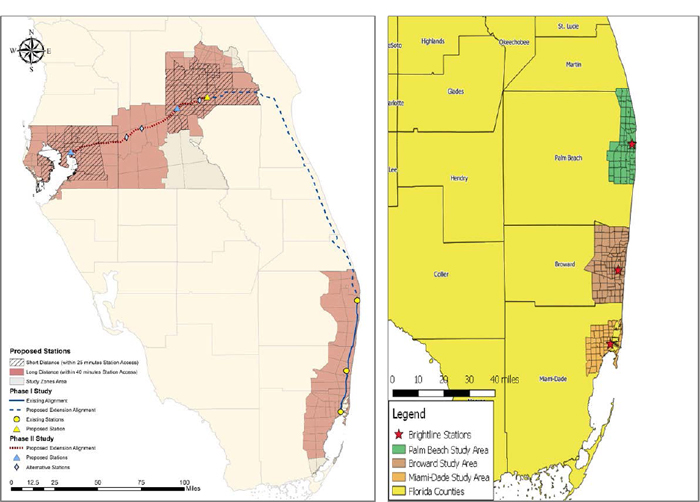
The earlier sections provided an overview of the regional socioeconomics in South and Central Florida and Tampa area. Following a review of the region, Louis Berger proceeded to identify the addressable market geography, or study area, for the Brightline service. This geography was determined based on the existing and proposed station locations as shown in Figure 1-1. The catchment area for long-distance intercity travel between Southeast Florida and Central Florida, between Southeast Florida and Lakeland and between Southeast Florida and Tampa was set to encompass an area within 30 to 40 minutes of driving time of a Brightline station. The catchment areas for shorter distance trips between Central Florida, Lakeland and Tampa area was set to encompass and areas within 20 to 30 minutes of drive time to the stations.
Source: Louis Berger, 2018
| 37 | P a g e |
Based on the station access travel times presented in Figure 3-1, Louis Berger developed study areas for both long and short distance market segments in the Phase I and Phase II Studies (Figure 3-2). The shaded portion of the left side depicts 40 minute drive time to Brightline stations that defined the catchment areas of both Phase I and II long distance market areas. The cross hatched portion of the same figure depicts the 25 minute drive time to stations in the Tampa-Orlando corridor that was used to define the Phase II Study catchment area for short distance trips. The right portion of Figure 3-2 depicts the short distance travel market catchment areas for the Phase II Study that was drawn based on the regional travel demand models zonal structure to delineate 20 minute station access times.
| 3.2 | Travel Market for Brightline Phase I Study |
The Brighline Phase I provides service connecting between Central and Southeast Florida (long-distance trips) and connecting cities within Southeast Florida (short-distance trips), where travel currently takes place by bus, rail (Amtrak and Tri-tail), air and car.
| 3.2.1 | Bus |
Travel by bus is available for both short- and long-distance trips. Intercity buses take approximately 4-6 hours to travel between Central and Southeast Florida and make stops in all three Southeast Florida cities. Intercity buses also serve all city pairs in Southeast Florida, and a popular set of transit bus routes connects Miami with Fort Lauderdale via the I-95 Express Lanes.
| 38 | P a g e |
Historical and Current Market Size
The intercity bus operators serving the Central-Southeast Florida market include Florida Express, Greyhound, Florida Sunshine, Red Coach, Megabus, Jet Set Express, Smart Shuttle Line, SuperTours, and Javax. Louis Berger estimated an average of 35 daily departures per direction between Central and Southeast Florida in 2017 based on published bus schedules of all the operators listed above. Assuming an average of 20 passengers per vehicle and an O-D distribution pattern similar to that of the rail travel market, Louis Berger estimated the 2016 daily volumes presented in Table 3-1.
Table 3-1 Estimated Daily Intercity Long-Distance Bus Person Trips
| City Pair | 2010 | 2016 | 2010-2016 CAGR |
| Orlando to Miami | 212 | 297 | +5.8% |
| Orlando to Fort Lauderdale | 126 | 193 | +7.4% |
| Orlando to West Palm Beach | 145 | 209 | +6.3% |
| Total | 483 | 700 | +6.4% |
| Source: Louis Berger, 2017 |
The number of intercity bus connections in Southeast Florida is limited to one public agency and a small number of privately operated services, which make local stops in the three Southeast Florida cities on the way to further destinations, primarily Orlando and Tampa. Broward County Transit (BCT) operates the 95Express and 595Express services. Each offer approximately 30 buses per day per direction and attract a total of approximate 1,650 riders per day (average annual daily basis from BCT reports). The full one-way fare is $2.65. This service is growing rapidly – as of 2014, the service carried only approximately 1,000 riders per day (average annual daily basis from BCT reports). Services on private operators cost in the $10-$25 range for a one-way trip between Southeast Florida cities. Greyhound offers about 13 daily trips from Miami to Fort Lauderdale and six from Miami through to West Palm Beach. Other intercity bus operators serving the Southeast Florida market include Florida Express, Florida Sunshine, Red Coach, and Megabus.
Bus ridership estimates in Southeast Florida were developed by assuming 30 riders per bus within the short-distance market (with 27 bus departures per day serving this corridor) and an O-D distribution pattern similar to the commuter rail market within the same corridor. Published ridership estimates obtained from Broward County Transit were also added to the initially estimated volume of bus trips within the Fort Lauderdale-Miami city pair. Table 3-2 shows the number of bus riders assumed for the base year forecast.
Table 3-2 Estimated Daily Short-Distance Bus Person Trips
| City Pair | 2016 |
| W. Palm Beach – Fort Lauderdale | 277 |
| W. Palm Beach – Miami | 184 |
| Fort Lauderdale – Miami | 2,006 |
| Total | 2,468 |
| Source: Louis Berger, 2017 |
| 39 | P a g e |
Growth Forecast
Future-year bus ridership volumes were estimated by applying growth rates obtained from the Chaddick Institute for Metropolitan Development at DePaul University, which monitors intercity bus travel patterns in the country.3 The initial surge in intercity bus travel growth observed since 2007 has slowed in recent years – as shown in Figure 3-3. As such, Louis Berger applied a 1.7% CAGR to estimate future-year bus ridership, as shown in Table 3-3 and Table 3-4.
Figure 3-3 Historical Growth in Intercity Bus Travel in the United States
![]()
Source: Louis Berger analysis of data from the Chaddick Institute, 2016
Table 3-3 Projected Daily Intercity Long-Distance Bus Person Trips
| City Pair | 2016 | 2040 | 2016-2045 CAGR |
| Central Florida to Miami | 297 | 478 | |
| Central Florida to Fort Lauderdale | 193 | 311 | |
| Central Florida to West Palm Beach | 209 | 337 | |
| Total | 700 | 1,125 | +1.7% |
| Source: Louis Berger, 2017 |
Table 3-4 Projected Daily Short-Distance Bus Person Trips
| City Pair | 2016 | 2045 |
2016-2045 CAGR |
| W. Palm Beach to Fort Lauderdale | 277 | 446 | |
| W. Palm Beach to Miami | 184 | 296 | |
| Fort Lauderdale to Miami | 2,006 | 3,225 | |
| Total | 2,468 | 3,967 | +1.7% |
| Source: Louis Berger, 2017 |
3 “The Remaking of the Motor Coach: 2015 Year in Review of Intercity Bus Service in the United States”, Chaddick Institute for Metropolitan Development at DePaul University, January 2016, https://las.depaul.edu/centers-and-institutes/chaddick-institute-for-metropolitan-development/research-and-publications/Documents/2015%20Year%20in%20Review%20of%20Intercity%20Bus%20Service%20in%20the%20Unite d%20States.pdf
| 40 | P a g e |
3.2.2 Long-Distance Rail (Amtrak)
The rail travel market analyzed in this study is separated into long- and short-distance markets. Amtrak provides services for the long-distance market, from Miami to Orlando twice a day. The Amtrak service makes 11 stops between Miami and Orlando, including Fort Lauderdale and West Palm Beach. In Miami, the Amtrak station is in Hialeah, approximately a 20-minute drive northwest of downtown. In Fort Lauderdale, the Amtrak station is on the west side of I-95, approximately a 10-minute drive west of downtown. In West Palm Beach, the Amtrak station is a short walk from the proposed Brightline station. In Orlando, the Amtrak station is downtown, approximately a 25-minute drive northwest from the airport.
Historical and Current Market Size
Boarding and alighting data for all Amtrak stations in Florida is presented in Figure 3-4, showing ridership to, within, and from the state fluctuating between 700,000 and 1.25 million trips annually. The fluctuations around an overarching trend of growth between 2003 and 2016 reflect shifts in economic conditions as well as competitive dynamics overall in the intercity travel market (fuel prices, growth in intercity bus travel, etc.).
Figure 3-4 Amtrak Florida Station Boardings
![]()
Source: National Association of Rail Passengers Amtrak Ridership Statistics, 2017
However, Amtrak ridership between Central and Southeast Florida is limited to only a relatively small portion of the total boardings and alightings statistics shown in Figure 3-4. Louis Berger estimated the proportion of Central to Southeast Florida trips using 2008 Amtrak station-pair ridership data. The resulting count is approximately 36,000 trips annually, as shown in the city-pair breakdown in Table 3-5. The 2016 intercity trip estimate uses the 2008 passenger trip distribution with some adjustments to account for changes in Amtrak Florida station boardings and alightings. The relatively small long-distance rail travel market is most likely a function of Amtrak’s high travel times.
| 41 | P a g e |
Growth Forecast
Louis Berger estimated future-year estimates of Amtrak ridership between Central and Southeast Florida by applying the growth rates implied by the trend projection in Figure 3-4, resulting in CAGR of 0.4%, as shown in Table 3-5.
Table 3-5 Historical and Future Amtrak Passenger Volumes
| City Pair | 2008 | 2016 | 2045 | 2016-2045 CAGR |
2045 Daily |
| Orlando – W. Palm Beach | 10,338 | 10,519 | 11,698 | +0.4% | 32 |
| Orlando – Fort Lauderdale | 9,946 | 9,711 | 10,800 | +0.4% | 30 |
| Orlando – Miami | 15,762 | 14,932 | 16,606 | +0.4% | 45 |
| Total | 36,046 | 35,162 | 39,105 | +0.4% | 107 |
| Source: Amtrak, National Association of Rail Passengers, Louis Berger, 2017 |
3.2.3 Short-Distance Rail (Tri-Rail)
While the Amtrak service can be used for travel within Southeast Florida, the short-distance rail market is primarily served by Tri-Rail, a commuter rail line managed by the South Florida Regional Transportation Authority (SFRTA) connecting Miami and West Palm Beach, making a total of 18 station stops over 72 miles. The system has 5 stations in Miami-Dade County, 7 in Broward County, and 6 in Palm Beach County, as shown in Figure 3-5. This service runs 15 times a day per direction. In all three cities, shuttle connections are provided to the airports. In Miami, connection is available to Metrorail at the Metrorail Transfer station, whereas in Fort Lauderdale and West Palm Beach, Amtrak and Tri-Rail share a station. Tri-Rail’s southernmost station is near the Miami airport, approximately a 20 minute drive northwest of downtown. A planned extension of the Tri-Rail system will offer direct connectivity from MIA to Brightline’s Miami Central Station.
| 42 | P a g e |
Figure 3-5 Tri-Rail System Map
![]()
Source: Tri-Rail System Map
Figure 3-6 shows annual system ridership obtained from the Tri-Rail monthly operation statistics and the National Transit Database (NTD). System ridership has grown at an annualized rate of 2.9% over the last ten years, although that rate of growth appears to be slowing down (1.2% annualized rate of growth over the last five years).
| 43 | P a g e |
Figure 3-6 Tri-Rail System Ridership
![]()
Source: National Transit Database
Only the relevant stations that provide an alternative to Brightline based on origins and destinations were included in the Tri-Rail ridership estimates. Primary stations covered by the three Brightline service short-distance markets in West Palm Beach, Fort Lauderdale, and Miami, respectively, were:
| ● | Mangonia Park Station, West Palm Beach, and Lake Worth; |
| ● | Fort Lauderdale downtown, Fort Lauderdale Airport, and Sheridan St.; and |
| ● | Opa-Locka, Metrorail Transfer Station, Hialeah Market, and Miami Airport. |
Growth Forecast
Louis Berger examined the South Florida Regional Transportation Authority’s SFRTA Forward Plan: A Transit Development Plan for SFRTA FY 2014-2023. This report contained the results of a 2013 on-board and platform intercept origin and destination survey for Tri-Rail that can be used to determine the portion of Tri-Rail ridership traveling between the three cities to be served by Brightline. The survey indicated that approximately 24 percent of total ridership has both an origin and destination in the central city locations to be served by Brightline. Table 3-6 presents the estimate of applicable Tri-Rail ridership by city pair. The 2045 estimates reflect the growth implied by the trend presented in Figure 3-6.
Table 3-6 Current and Projected Daily Short-Distance Rail Trips
| City Pair | 2016 | 2045 | CAGR | Daily (2045) |
| Miami – West Palm Beach | 229,807 | 300,607 | +0.9% | 824 |
| Miami – Fort Lauderdale | 434,227 | 568,006 | +0.9% | 1,556 |
| Fort Lauderdale – West Palm Beach | 345,636 | 452,122 | +0.9% | 1,239 |
| Total | 1,009,671 | 1,320,735 | +0.9% | 3,618 |
|
Source: Louis Berger, 2017
|
| 44 | P a g e |
3.2.4 Air
Air travel is available at two airport pairs for travel from Southeast Florida to Central Florida. From Orlando International Airport (IATA airport code MCO), flights are available to Fort Lauderdale-Hollywood International Airport (IATA code FLL – via Spirit and Silver Airways) and Miami International Airport (IATA code MIA – via American and Delta). Currently, no flights from Central Florida are available to Palm Beach International Airport (IATA code PBI).
Historical and Current Market Size
Air travel volumes for the long-distance travel market were derived using data obtained from the FAA 10% sample of tickets, and corroborated against the Orlando International Airport air traffic reports published by Greater Orlando Aviation Authority (GOAA). Louis Berger compiled and reviewed historical data from the Federal Aviation Authority’s (FAA) 10 percent sample of tickets database. This data was used to trace historical volumes of air travel between each of the city pairs that offer air travel.
Historical air traffic data going back twenty years in Figure 3-7 shows a general decline air passenger volumes between Central and Southeast Florida, largely accelerated by the additional airport security requirements instituted after the events of September 11, 2001. Air traffic volumes post the 9-11 declines in short-distance air travel have remained relatively steady with fluctuations reflecting the effects of economic conditions.
Figure 3-7 Annual Air Traffic Volume between Central and Southeast Florida
![]()
Source: FAA 10 Percent Tickets Database, 2017
| 45 | P a g e |
Figure 3-7 shows that air passenger traffic between MCO and MIA has steadily grown post 9-11 while the volumes of trips between MCO and FLL have steadily declined, and trips between MCO and PBI have declined to zero. Table 3-7 shows the change in trip volumes between 2010 and 2016 by airport pair in both annual and daily terms.
Table 3-7 Annual Air Passenger Volumes, FAA 10% Ticket Sample
| Airport Pair (Both Directions) | 2010 | 2010 | 2016 | 2016 | 2010-2016 |
| Annual | Daily | Annual | Daily | CAGR | |
| Orlando (MCO) – WPB (PBI) | 40 | <1 | 0 | 0 | |
| Orlando(MCO) – Fort Lauderdale (FLL) | 163,500 | 448 | 54,880 | 150 | -16.7% |
| Orlando (MCO) – Miami (MIA) | 88,900 | 244 | 168,050 | 460 | +11.1% |
| Total | 252,440 | 692 | 222,930 | 610 | -2.1% |
|
Source: Louis Berger, 2017
|
Growth Forecast
Given the trends depicted in Figure 3-7, Louis Berger estimated the future growth of the Central to Southeast Florida travel market based on the FAA’s Terminal Area Forecasts (TAF) for all three airports (MCO, FLL and MIA). TAF is the official forecast of aviation activity at U.S. Airports and are econometrically driven demand-side forecasts.
Figure 3-8 compares Central to Southeast Florida air passenger volumes against the volume of total enplanements at the three airports. The figure shows that the share air passenger traffic between Central and Southeast Florida has been declining relative to the total volume of air passenger enplanements at all three airports. The study team applied this trend of declining shares to the TAF projected growth in enplanements at all three airports.
Figure 3-8 Comparison of Air Traffic Volumes
![]()
Source: FAA Terminal Area Forecast, 2016
| 46 | P a g e |
The resulting volume of air passenger traffic between Central and Southeast Florida was further segmented to distinguish between travel to Fort Lauderdale and Miami based on the trends presented in Figure 3-5. Table 3-8 presents the resulting estimates of air passengers in the Brightline service travel market. The resulting air passenger volumes in the Central to Southeast Florida market grow at about a third of the rate projected for total enplanements of study area airports. This positive growth is attributed to growth observed within the Orlando-Miami city pair.
Table 3-8 Estimates of Air Passengers in the Brightline Service Travel Market
| 2002 Annual |
2010 Annual |
2016 Annual |
2045 Annual |
2045 Daily | 2016-2045 CAGR |
|
| Total Enplanements (MCO/FLL/MIA) | 21,798,554 | 27,180,107 | 34,861,631 | 62,033,916 | 169,840 | +2.01% |
| Orlando (MCO) – Fort Lauderdale (FLL) | 205,240 | 163,500 | 54,880 | 40,304 | 110 | -1.06% |
| Orlando (MCO) – Miami (MIA) | 68,380 | 88,900 | 168,050 | 231,391 | 634 | +1.11% |
| Central Florida – Southeast Florida | 273,620 | 252,400 | 222,930 | 271,695 | 744 | +0.68% |
| % of Enplanements | 1.26% | 0.93% | 0.64% | 0.44% |
Source: Louis Berger, 2017
3.2.5 Auto
Auto is the prevalent mode of travel within Southeast Florida and the dominant mode of travel between Southeast and Central Florida. Two primary auto routes collect a significant majority of traffic between Southeast Florida and Central Florida – the Florida Turnpike and I-95. While the Florida Turnpike is faster and more direct, it is a toll road, whereas I-95 is a free route. The two other highway routes between the two regions – US-27 and I-75 – add one and two hours respectively to the travel time between the two regions. Southeast Florida has a dense and often significantly congested highway network, but the Florida Turnpike and I-95 remain the major north-south arteries connecting the three Southeast Florida cities under discussion in this report. Other north-south arteries are either signaled (US-1, US-441) or further inland (SR-826, I-75, Florida Turnpike Homestead Extension).
Historical and Current Market Size
Louis Berger reviewed historical traffic counts on the Florida Turnpike and I-95 at points in between Southeast Florida and Central Florida, and found significant growth over the past decades. Traffic on the Florida Turnpike represents about 80% of the total traffic volume between Central and Southeast Florida. Louis Berger identified two counter stations on the Florida Turnpike between West Palm Beach and Orlando that are representative of the traffic traveling on the Turnpike between Central and Southeast Florida. Traffic on these stations has grown at a 3.2% CAGR from 2001 to 2016, with a slight decline during the years of the Great Recession. On I-95, which represents about 20% of the total traffic volume traveling between Central and Southeast Florida, the traffic counter in St. Lucie, FL – an intermediate point between the main urban areas of Orlando and West Palm Beach – indicates an average annual traffic growth of approximately 2.1% from 2001 to 2015. Annual traffic counts at four counters on the major roads connecting Southeast Florida and Central Florida, including the two counters discussed above, are shown in Figure 3-9 and Figure 3-10.
| 47 | P a g e |
Figure 3-9 Florida Turnpike Central-to-Southeast Florida Historical Traffic Counts
![]()
Source: Louis Berger analysis of data from FDOT, 2017
Figure 3-10 I-95 Central-to-Southeast Florida Historical Traffic Counts
![]()
Source: Louis Berger analysis of data from FDOT, 2017
Current traffic flows between Central and Southeast Florida on the Turnpike and I-95 are characterized as follows:
| ● | Day of week patterns – Friday is the busiest day at all four counters, with average traffic on Friday being 21% above the average day. Tuesdays and Wednesdays are the least busy days at all four counters. The prominence of weekends is particularly pronounced at the Turnpike counters, where Friday-Saturday traffic counts are 17% above the average day. Furthermore, the Turnpike counters exhibit directionality on the weekends, with 38% more traffic seen on Sundays in the northbound direction than southbound, |
| 48 | P a g e |
| and with 21% less traffic seen on Sundays in the northbound direction than southbound. Similar, but more muted, effects are seen on Mondays, Thursdays, and Saturdays, as well as on I-95 on Fridays and Sundays. |
| ● | Time of day patterns – From investigating hourly traffic counter data from June 2016, the four counters appear to behave fairly idiosyncratic travel patterns by time of day. The St. Lucie County counter on the Florida Turnpike peaks at roughly midday every day of the week in both directions of travel. The St. Lucie County counter on I-95 displays traditional peaking (with weekday peaks in the morning and afternoon, and weekend peaks at midday), but traffic levels appear higher at the afternoon weekday peak in both directions than in the morning peak. The Osceola County counter on the Florida Turnpike displays traditional peaking, with weekday morning peak traffic heading northbound, and weekday afternoon peak traffic heading southbound. At all counters, the highest-traffic hours tend to each represent roughly 8.5% of daily traffic. |
| ● | Type of vehicle– The split of traffic by vehicle type are broadly similar across the counters, as well as by year through the 2001-2016 time period. Passenger vehicles represent roughly 85% of traffic, whereas trucks represent roughly 15% of traffic. The 15% of traffic represented by trucks is composed roughly of 4% single-unit trucks, 10% combination trailer trucks, and 1% multi-trailer trucks. |
Accurately evaluating historical traffic growth within the three Southeast Florida cities is more complex, since there are a significant amount of potential origins and destinations in between the three main cities and therefore an important number of local trips that cannot be accurately accounted for. In order to gain an indication of the number of historical trips, Louis Berger investigated traffic counters between the three Southeast Florida cities on both I-95 and the Florida Turnpike, using FDOT’s Florida Traffic Online web portal. The AADTs at the four counters are shown in Figure 3-11 and Figure 3-12. From 2001 to 2016, traffic grew more quickly at both Florida Turnpike counters (2.8% CAGR at Atlantic Ave. and 3.7% at SR-824) than at the I-95 counters (0.6% at SR-858 and 0.3% at 48th St.), a pattern which can be explained by a combination of growing incomes in Southeast Florida and capacity issues on I-95. Traffic on both main routes, however, indicates an upward trajectory.
| 49 | P a g e |
Figure 3-11 Southeast Florida Historical Traffic Counts
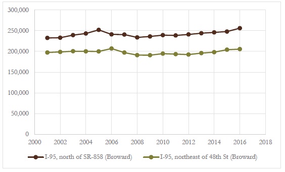
Source: Louis Berger analysis of data from FDOT, 2017
Figure 3-12 Southeast Florida Historical Traffic Counts
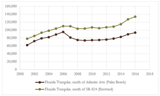
Source: Louis Berger analysis of data from FDOT, 2017
Louis Berger relied on cell-phone data to establish the size of the current auto market for both long- and short- distance trips. Datasets purchased from AirSage, a company specialized in collecting and analyzing cell-phone location data, included observed travel behavior for March, June, September, and December of 2016. This dataset included all trips between origin and destination zones within the addressable geographic market for Brightline (Section 2.10).
| 50 | P a g e |
For trips seen in the cell-phone movement datasets, AirSage increments the trip table for the origin-destination pair based on a factor dependent on the population estimate and cell-phone penetration of that device’s home location (which is determined by an algorithm based on the device’s nighttime location). Population estimates are consistent with US Census data estimates. Based on this home location, AirSage also allocates the resulting trips to either a “resident” or a “visitor” category. Any device whose home location is outside of the zones included in the addressable geographical market for Brightline is classified as a “visitor”. The AirSage data also reflects all trips regardless of mode.
In order to ensure that the data is representative of the auto market within the addressable market geography for Brightline, Louis Berger had to perform the following adjustments to the AirSage data:
| ● | Deduct trips from other modes as such that the data represents auto trips only, using the existing market size estimates for each mode described earlier in this section. |
| ● | For short-distance trips, reducing the number of trips by 12% to account for the percentage of travelers manifesting the need to use a car for intermediate stops during their trips, as indicated in the 2012 Stated Preference Survey (See Section 4.2.1). This percentage of travelers are considered to be captive to the auto mode choice, and are therefore not considered part of the in-scope market for Brightline. |
| ● | For long-distance trips, the visitor market was initially reduced by 46% in market size to calibrate the trip counts to vehicle counts observed on the Florida Turnpike; and then further revised down by 25% to account for through trips whose origin or destination is not within the addressable market geography. |
Table 3-9 shows the resulting average daily travel counts for the long-distance market, while Table 3-10 shows the resulting average daily travel counts for the short-distance market.
Table 3-9 Estimated Daily Long-Distance Auto Person Trips
| City Pair | Resident SB |
Resident NB |
Resident Total |
Visitor SB |
Visitor NB | Visitor Total |
Total |
| Orlando to West Palm Beach | 12,473 | 12,236 | 24,710 | 2,652 | 2,658 | 5,310 | 30,019 |
| Orlando to Fort Lauderdale | 8,083 | 7,764 | 15,846 | 2,066 | 2,050 | 4,116 | 19,962 |
| Orlando to Miami | 8,400 | 8,139 | 16,538 | 2,088 | 1,943 | 4,031 | 20,569 |
| Total | 28,955 | 28,139 | 57,094 | 6,806 | 6,651 | 13,457 | 70,551 |
Source: Louis Berger analysis of AirSage data, 2017. SB = Southbound; NB = Northbound
Table 3-10 Estimated Daily Short-Distance Auto Person Trips
| City Pair | Resident SB |
Resident NB |
Resident Total |
Visitor SB |
Visitor NB | Visitor Total |
Total |
| West Palm Beach to Miami | 11,641 | 11,699 | 23,339 | 22,909 | 20,743 | 43,651 | 66,991 |
| W.P.B. to Fort Lauderdale | 88,047 | 88,181 | 176,228 | 100,207 | 101,610 | 201,817 | 378,044 |
| Fort Lauderdale to Miami | 147,939 | 151,424 | 299,363 | 131,413 | 128,243 | 259,657 | 559,019 |
| Total | 247,626 | 251,304 | 498,930 | 254,529 | 250,596 | 505,125 | 1,004,055 |
Source: Louis Berger analysis of AirSage data, 2017
Table 3-11 shows the share of trips allocated to each city pair for residents and visitors in the long-distance travel market while Table 3-12 shows the same statistic, but for the short-distance travel market. As shown, the three city pairs have roughly equal shares in the long-distance market, with Orlando-West Palm Beach holding a slight plurality. In the short-distance market, the Fort Lauderdale-Miami city pair dominates.
| 51 | P a g e |
Table 3-11 Long-Distance City Pair O-D Shares
| City Pair | Resident | Visitor | Total |
| Orlando to West Palm Beach | 43% | 39% | 43% |
| Orlando to Fort Lauderdale | 28% | 31% | 28% |
| Orlando to Miami | 29% | 30% | 29% |
|
Source: Louis Berger, 2017
|
Table 3-12 Short-Distance City Pair O-D Shares
| City Pair | Resident | Visitor | Total |
| West Palm Beach to Miami | 5% | 9% | 7% |
| W.P.B. to Fort Lauderdale | 35% | 40% | 38% |
| Fort Lauderdale to Miami | 60% | 51% | 56% |
|
Source: Louis Berger, 2017
|
Growth Forecast
In order to estimate future growth for the long-distance auto travel market, Louis Berger developed an econometric model of traffic on the Florida Turnpike. The model used historical monthly traffic counts for the 2001-2016 period for a traffic counter station located at a point north of SR-70 on the Florida Turnpike. The economic variables considered included employment, number of households, and gas prices. Seasonal variation by month of year was also taken into account in the model development. This monthly count data also served as a validation of the long-distance origin-destination trip estimates provided by AirSage.
The traffic model specification was evaluated by comparing fitted versus actual traffic over the recent historical period going back to January of 2001 as shown in Figure 3-13. The resulting close agreement between fitted and actual model results provides confidence in the model’s ability to map key drivers to actual traffic levels. Figure 3-14 presents the historical observed and forecast traffic of Central – Southeast Florida Turnpike Traffic. Traffic at the counter grew at a 3.2% CAGR. The econometric model forecasts a 3.2% CAGR through 2047. Additional information on the traffic model, including sources and forecasts for the economic variables used, can be found in Appendix B.
| 52 | P a g e |
Figure 3-13 Florida Turnpike Traffic Model Performance (Actual Vs. Fitted – Monthly)
![]()
Source: Louis Berger analysis, 2017
Figure 3-14 Econometric Analysis and Projection of Florida Turnpike Traffic (Monthly)
![]()
Source: Louis Berger analysis, 2017
Growth estimates for the short-distance market are based on the growth rates modeled in the Southeast Florida Regional Planning Model (SERPM), maintained by the Florida Department of Transportation. This regional planning
| 53 | P a g e |
model accounts for a 1.2% annual growth rate in travel in the Southeast Florida region, broadly in line with regional employment growth forecasts discussed in Section 2.5.
3.3 Travel Market for Brightline Phase II Study
The Brighline Phase II provides service connecting between Tampa Area and Southeast Florida (long-distance trips), where travel currently takes place by bus, rail (Amtrak), air, and car, and connecting cities within Tampa Area, Lakeland and Central Florida (short-distance trips), where travel mainly takes place by bus and car. Because Brighline Phase II will include a terminal station at Orlando Airport, Louis Berger team also analyzed travel market for airport access trips in addition to non-airport trips (short- and long-distance trips)
3.3.1 Bus
Travel by bus is available for both short- and long-distance trips. Long-distance intercity buses take approximately 3-6 hours to travel within study area. Short-distance intercity buses also serve all city pairs in Central Florida, Tampa and Lakeland area.
Current Market Size
The intercity bus operators serving the study area market include Florida Express, Greyhound, Florida Sunshine, Red Coach, Megabus, Jet Set Express, Smart Shuttle Line, SuperTours, and Javax. Louis Berger estimated an average of 43 daily departures per direction between Central and Southeast Florida in 2017, when this study was conducted, based on published bus schedules of all the operators listed above. Assuming an average of 30 passengers per vehicle and an O-D distribution pattern similar to that of the rail travel market, Louis Berger estimated the 2018 daily volumes presented in Table 3-13; Louis Berger also compared the estimates with those provided by Developing Refined Estimates of Intercity Bus Ridership (Prepared by RSG).
Table 3-13 Estimated Daily Intercity Long-Distance Bus Person Trips
| City Pair | Daily | Weekly | Weekly RSG Benchmark |
| Tampa - Orlando | 158 | 1,103 | n/a |
| Lakeland - Orlando | 11 | 77 | n/a |
| Tampa - Lakeland | 11 | 80 | n/a |
| Tampa Area-Southeast Florida | 240 | 1,680 | 500-1999 |
|
Tampa - West Palm Beach
|
82 | 577 | |
|
Tampa - Ft Lauderdale
|
56 | 395 | |
|
Tampa - Miami
|
101 | 708 | |
| Lakeland Area-Southeast Florida | 60 | 420 | n/a |
|
Lakeland - West Palm Beach
|
18 | 127 | n/a |
|
Lakeland - Ft Lauderdale
|
16 | 112 | n/a |
|
Lakeland - Miami
|
26 | 181 | n/a |
| Total | 480 | 3,360 | n/a |
| Source: Louis Berger, 2018 and Developing Refined Estimates of Intercity Bus Ridership, RSG, 2015 | |||
| 54 | P a g e |
Figure 3–15 Ridership Benchmark FromRSG
![]()
Source: Louis Berger, 2018 and Developing Refined Estimates of Intercity Bus Ridership, RSG, 2015
Growth Forecast
Future-year bus ridership volumes were estimated by applying growth rates of population obtained from the Bureau of Economic and Business Research (BEBR) at University of Florida. The growth rates were based on BEBR Medium case and were considered in each study area separately.
Table 3–14 Projected Daily Intercity Bus Person Trips
| City Pair | 2017 | 2045 | CAGR |
| Tampa - Orlando | 158 | 223 | 1.2% |
| Lakeland - Orlando | 11 | 15 | 1.1% |
| Tampa - Lakeland | 11 | 17 | 1.6% |
| Tampa Area-Southeast Florida | 239 | 310 | 0.9% |
| Tampa - West Palm Beach | 82 | 107 | 1.0% |
| Tampa - Ft Lauderdale | 56 | 71 | 0.9% |
| Tampa - Miami | 101 | 132 | 1.0% |
| Lakeland Area-Southeast Florida | 60 | 78 | 0.9% |
| Lakeland - West Palm Beach | 18 | 24 | 1.0% |
| Lakeland - Ft Lauderdale | 16 | 20 | 0.8% |
| Lakeland - Miami | 26 | 34 | 1.0% |
| Total | 480 | 643 | 1.1% |
| Source: Louis Berger, 2018 |
| 55 | P a g e |
3.3.2 Rail (Amtrak)
Amtrak provides services from Tampa to Southeast Florida via Orlando. The Amtrak service makes 8 major stops within the study area, including Tampa, Lakeland, Winter Haven, Winter Park, Orlando, West Palm Beach, Fort Lauderdale and Miami.
Historical and Current Market Size
Boarding and alighting data for all Amtrak stations in Florida is presented in Figure 3-16, showing ridership to, within, and from the state fluctuating between 700,000 and 1.25 million trips annually. The fluctuations around an overarching trend of growth between 2003 and 2017 reflect shifts in economic conditions as well as competitive dynamics overall in the intercity travel market (fuel prices, growth in intercity bus travel, etc.).
Figure 3–16 Amtrak Florida Station Boardings (Thousands)
![]()
Source: National Association of Rail Passengers Amtrak Ridership Statistics, 2017
Growth Forecast
Louis Berger estimated future-year estimates of Amtrak ridership between Central and Southeast Florida by applying the growth rates implied by the trend projection in Figure 3-16, resulting in CAGR of 1.1%, as shown in Table 3-15.
Table 3–15 Historical and Future Amtrak Passenger Volumes
| City Pair | 2008 | 2017 | 2045 | 2017-2045 CAGR |
2045 Daily |
| Tampa - Orlando | 11,832 | 11,762 | 16,235 | 1.2% | 44 |
| Lakeland - Orlando | 879 | 818 | 1,062 | 0.9% | 3 |
| Tampa - Lakeland | 828 | 857 | 1,231 | 1.3% | 3 |
| Tampa Area-Southeast Florida | 36,580 | 38,191 | 55,435 | 1.3% | 152 |
| Tampa - West Palm Beach | 11,825 | 13,116 | 19,295 | 1.4% | 53 |
| Tampa - Ft Lauderdale | 8,570 | 8,972 | 13,258 | 1.4% | 36 |
| Tampa - Miami | 16,185 | 16,103 | 22,882 | 1.3% | 63 |
| Lakeland Area-Southeast Florida | 20,705 | 18,906 | 24,551 | 0.9% | 67 |
| Lakeland - West Palm Beach | 5,700 | 5,719 | 7,605 | 1.0% | 21 |
| Lakeland - Ft Lauderdale | 5,593 | 5,043 | 6,657 | 1.0% | 18 |
| Lakeland - Miami | 9,412 | 8,144 | 10,289 | 0.8% | 28 |
| Total | 70,824 | 70,534 | 98,514 | 1.2% | 270 |
Source: Amtrak, National Association of Rail Passengers, Louis Berger, 2018
| 56 | P a g e |
3.3.3 Air
Air travel is available from Tampa to Southeast Florida with flights between Tampa International Airport (TPA) to both Fort Lauderdale and Miami airports.
Historical and Current Market Size
Similar to the discussion of the air travel market in Section 3.2, air travel volumes for the Phase II Study were derived using data obtained from the FAA 10% sample of tickets. Figure 3-17 shows the historical volume of origin-destination (O-D) air travel between Tampa (TPA) and both Fort Lauderdale (FLL) and Miami (MIA). Similar to the patterns observed in the Orlando to Southeast Florida market, this figure shows a declining trend of air passenger volumes to and from Fort Lauderdale, and conversely, an increasing trend of air passenger volumes to and from Miami.
Figure 3–17 Annual Air Traffic Volume between Tampa and Southeast Florida
![]()
Source: FAA 10 Percent Tickets Database, 2018
Table 3-16 shows the change in trip volumes between 2010 and 2017 by airport pair in both annual and daily terms.
Table 3–16 Annual Air Passenger Volumes, FAA 10% Ticket Sample
| Airport Pair (Both Directions) | 2010 Annual |
2010 Daily |
2017 Annual |
2017 Daily |
2010-2017 CAGR |
| Tampa Area-Southeast Florida | 347,300 | 952 | 384,650 | 1,054 | 1.47% |
|
Tampa (TPA) – Fort Lauderdale (FLL)
|
265,980 | 729 | 220,320 | 604 | -2.65% |
|
Tampa (TPA) – Miami (MIA)
|
81,320 | 223 | 164,330 | 450 | 10.57% |
| 57 | P a g e |
Growth Forecast
Given the trends depicted in Figure 3-17, Louis Berger estimated the future growth of the Tampa-Southeast Florida travel market by determining the share of this travel market in relation to the overall air travel activity at all three airports. Figure 3-18 depicts both the historical and projected levels of enplanements at both airports obtained from the FAA’s Terminal Area Forecasts (TAF) for all three airports (TPA, FLL and MIA). All of these three airports experienced significant growth in enplanements over the past 30 years and are expected to continuing grow along similar trajectories over the next 30 years. Figure 3-19 depicts the historical and projected trends of TPA-FLL and TPA-MIA volumes. Based on this assessment, Louis Berger predicted the growth in air travel that is depicted in Figure 3-20.
Figure 3–18 FAA’s Terminal Area Forecasts For Airport Enplanements In Study Area
![]()
Source: FAA Terminal Area Forecast, 2018
| 58 | P a g e |
Figure 3–19 Passenger Volume Share Of Enplanement In Origin And Destination Airport
![]()
Source: Louis Berger, 2018
Figure 3–20 Prediction Of Future Passenger Volume Between City Pairs
![]()
Source: Louis Berger, 2018
3.3.4 Auto
Auto is the prevalent mode of travel within Southeast Florida and the dominant mode of travel with study area. Two primary auto routes collect a significant majority of traffic between Southeast Florida and Central Florida – the Florida Turnpike and I-95. While the Florida Turnpike is faster and more direct, it is a toll road, whereas I-95 is a free route.
| 59 | P a g e |
The two other highway routes, I-4 and I-75, connect Tampa and Southeast Florida and Tampa and Central Florida separately.
Historical and Current Market Size
Louis Berger reviewed historical traffic counts on the Florida Turnpike, I-9, I-4 and I-75 at points within study area, and found significant growth over the past decades. Traffic on the Florida Turnpike represents about 80% of the total traffic volume between Central and Southeast Florida. Louis Berger identified four counter stations on these four routes that are representative of the traffic traveling from Central Florida and Tampa to Southeast Florida and from Tampa to Central Florida. Traffic on these stations has grown at a 3.1% CAGR from 2002 to 2017, with a slight decline during the years of the Great Recession. Annual traffic counts at four counters on the major roads connecting Southeast Florida and Central Florida, including the two counters discussed above, are shown in Figure 3-21 and Figure 3-22.
| 60 | P a g e |
Figure 3–21 Counter stations identified for historical traffic volume
![]()
Source: Louis Berger, 2018
| 61 | P a g e |
Figure 3–22 Historical AADT Trend At Counter Stations
![]()
Source: Louis Berger, 2018
Table 3–17 Summary Of Historical Aadt And Cagr
|
Counter Stations
|
2002 | 2007 | 2012 | 2017 | 2002-2017 CAGR |
|
Turnpike
|
22,900 | 28,900 | 26,000 | 33,900 | 2.6% |
|
I-95
|
42,500 | 52,289 | 46,500 | 61,831 | 2.5% |
|
I-75
|
18,351 | 21,141 | 19,444 | 24,968 | 2.9% |
|
I-4
|
55,000 | 74,000 | 76,500 | 94,000 | 3.6% |
|
Total
|
136,000 | 145,100 | 154,294 | 165,585 | 3.1% |
Source: Louis Berger, 2018
Louis Berger relied on cell-phone data to establish the size of the current auto market of the study area. Datasets purchased from AirSage, a company specialized in collecting and analyzing cell-phone location data, included observed travel behavior for March, June, September, and December of 2017. This dataset included all trips between origin and destination zones within the travel market for Brightline.
| 62 | P a g e |
For trips seen in the cell-phone movement datasets, AirSage increments the trip table for the origin-destination pair based on a factor dependent on the population estimate and cell-phone penetration of that device’s home location (which is determined by an algorithm based on the device’s nighttime location). Population estimates are consistent with US Census data estimates. Based on this home location, AirSage also allocates the resulting trips to either a “resident” or a “visitor” category. Any device whose home location is outside of the zones included in the addressable geographical market for Brightline is classified as a “visitor”. The AirSage data also reflects all trips regardless of mode.
In order to ensure that the data is representative of the auto market within the addressable market geography for Brightline, Louis Berger had to perform the following adjustments to the AirSage data:
| ● | Deduct trips from other modes as such that the data represents auto trips only, using the existing market size estimates for each mode described earlier in this section. |
| ● | For short-distance trips, reducing the number of trips by 12% to account for the percentage of travelers manifesting the need to use a car for intermediate stops during their trips, as indicated in the 2012 Stated Preference Survey (See Section 4.2.1). This percentage of travelers are considered to be captive to the auto mode choice, and are therefore not considered part of the in-scope market for Brightline. |
| ● | For long-distance trips, the visitor market was initially reduced by 46% in market size to calibrate the trip counts to vehicle counts observed on the Florida Turnpike; and then further revised down by 25% to account for through trips whose origin or destination is not within the addressable market geography. |
Table 3–18 Estimated Daily Auto Person Trips By Time Of Day
|
Resident
|
Visitor |
Total | |||||||||
| City Pair | AM | MD |
PM
|
NT | Total | AM | MD | PM | NT | Total | |
| Tampa - Orlando | 2,514 | 16,119 | 8,371 | 11,547 | 38,551 | 832 | 8,080 | 3,836 | 5,738 | 18,486 | 57,037 |
| Lakeland - Orlando | 1,044 | 3,975 | 2,248 | 2,962 | 10,229 | 359 | 2,282 | 1,209 | 1,651 | 5,501 | 15,730 |
| Tampa - Lakeland | 1,025 | 4,756 | 2,454 | 3,480 | 11,715 | 226 | 1,773 | 924 | 1,271 | 4,194 | 15,909 |
| Tampa Area-Southeast Florida | 423 | 4742 | 2622 | 3019 | 10,806 | 155 | 1653 | 934 | 1058 | 3,800 | 14,606 |
| Tampa - West Palm Beach | 55 | 959 | 559 | 525 | 2,098 | 18 | 299 | 164 | 166 | 647 | 2,745 |
| Tampa - Ft Lauderdale | 169 | 1,596 | 848 | 960 | 3,573 | 71 | 602 | 314 | 367 | 1,354 | 4,927 |
| Tampa - Miami | 199 | 2,187 | 1,215 | 1,534 | 5,135 | 66 | 752 | 456 | 525 | 1,799 | 6,934 |
| Lakeland Area-Southeast Florida | 298 | 2210 | 1116 | 1388 | 5,012 | 101 | 743 | 364 | 475 | 1,683 | 6,695 |
| Lakeland - West Palm Beach | 112 | 762 | 397 | 422 | 1,693 | 34 | 248 | 107 | 141 | 530 | 2,223 |
| Lakeland - Ft Lauderdale | 81 | 653 | 327 | 394 | 1,455 | 30 | 213 | 102 | 128 | 473 | 1,928 |
| Lakeland - Miami | 105 | 795 | 392 | 572 | 1,864 | 37 | 282 | 155 | 206 | 680 | 2,544 |
| Total | 5,304 | 31,802 | 16,811 | 22,396 | 76,313 | 1,673 | 14,531 | 7,267 | 10,193 | 33,664 | 109,977 |
| % of Total Trips | 4.82% | 28.92% | 15.29% | 20.36% | 69.39% | 1.52% | 13.21% | 6.61% | 9.27% | 30.61% | 100.00% |
Source: Louis Berger, 2018
Growth Forecast
Louis Berger predicts future auto market based on AirSage data and applies average annual growth historical rate of growth at the relevant counter stations to make projections of future growth as shown in Table 3-19. The future auto market between key origins and destinations in the Phase 2 Study market will increase with CAGR of 2.0%.
| 63 | P a g e |
Table 3–19 Annual Auto Person Trips Projection
|
City Pair
|
2017 | 2045 | CAGR |
|
Tampa - Orlando
|
20,749,188 | 38,593,355 | 2.2% |
|
Lakeland - Orlando
|
5,735,777 | 10,668,509 | 2.2% |
|
Tampa - Lakeland
|
5,801,778 | 10,791,269 | 2.2% |
|
Tampa Area-Southeast Florida
|
4,821,022 | 9,109,907 | 2.3% |
|
Tampa - West Palm Beach
|
958,363 | 1,810,944 | 2.3% |
|
Tampa - Ft Lauderdale
|
1,548,900 | 2,926,834 | 2.3% |
|
Tampa - Miami
|
2,313,759 | 4,372,129 | 2.3% |
|
Lakeland Area-Southeast Florida
|
2,402,741 | 3,792,195 | 1.6% |
|
Lakeland - West Palm Beach
|
799,007 | 1,261,056 | 1.6% |
|
Lakeland - Ft Lauderdale
|
693,228 | 1,094,107 | 1.6% |
|
Lakeland - Miami
|
910,506 | 1,437,032 | 1.6% |
|
Total
|
39,510,506 | 72,955,235 | 2.2% |
|
Source: Louis Berger, 2018
|
3.3.5 Airport Access Trips
Sections above all discuss non-airport-access trips (intercity trips), which consist a majority of trips that can potentially be affected by introduction of Brightline Service. The Phase II Study also analyzed airport access trips to and from Orlando Airport given its proximity to Disney as well as to the other short distance market stations such as Tampa. The airport access trips include two categories--choice trips and captive trips-defined as below:
| ● | Captive trips- prepaid through travel packages etc |
| ● | Choice trips – travelers could choose from the array of options available including Brightline service. |
Louis Berger developed 2017 airport-access estimates trips based on data sourced from a 2002 Investment Grade Ridership Study prepared by AECOM and Wilbur Smith Associates for Florida High Speed Rail Authority. Further, Louis Berger team forecasts the future airport-access trips by applying growing trend of Disney visitation and MCO enplanements mentioned in the former sections. The current and future projections of airport access trips are choice trips presented in the table below:
| 64 | P a g e |
Table 3–20 Current And Future Airport Access Choice Trips By Mode
| 2017 | 2045 | 2017- 2045 CAGR |
|||||
| OD Pairs | Auto | Rental | Shuttle | Taxi | Total | Total | |
| Disney- MCO | 393,121 | 1,718,085 | 800,802 | 713,442 | 3,625,451 | 5,552,800 | 1.5% |
| Southwest Orlando (Excluded Disney)-MCO | 1,587,896 | 89,059 | 89,059 | 460,459 | 2,226,472 | 4,230,357 | 2.3% |
| Tampa-MCO | 635,269 | 35,630 | 35,630 | 184,216 | 890,745 | 1,692,439 | 2.3% |
| Lakeland-MCO | 193,718 | 10,865 | 10,865 | 56,175 | 271,623 | 516,090 | 2.3% |
| Total | 2,810,004 | 1,853,639 | 936,356 | 1,414,292 | 7,014,291 | 11,991,686 | 1.9% |
Source: Louis Berger, 2018
| 65 | P a g e |
| ● |
Primary market research. Data describing the travel patterns, behavior and attitudes of potential users of the service was collected through surveys, thereby providing the underlying basis for analyzing future ridership.
|
| ● |
Mode choice model estimation. Survey data was used to develop mathematical models of mode choice based on various modal service attributes and individual characteristics.
|
| ● |
Travel demand model development. Travel demand models were constructed for both long and short-distance travel. Service attributes of the various mode alternatives serving both markets were compiled and interacted with mode choice models to generate market share estimates under both build and no build conditions, thereby providing estimates of diversions to Brightline service.
|
| ● |
Screening Questions – Screening questions determine whether a person is qualified to participate in the survey.
|
| ● |
Reference trip – Data were collected to characterize the respondent’s most recent trip within the study area. Reference trip information included trip purpose; travel party composition; trip origin and destination; mode of travel.
|
| ● |
Choice Exercise – Respondents were presented with a series of hypothetical choice scenarios that include different travel options including Brightline. The reference trip described in previous questions is used to frame the hypothetical choice experiment.
|
| ● |
Induced Travel - It is expected that a portion of Brightline ridership will be trips that would not be made without Brightline. Respondents were asked about their interest in the additional intercity travel between Southeast and Central Florida and within Central Florida.
|
| ● |
Socioeconomic/demographic characteristics – Socioeconomic characteristics include age, gender, household size, household income, education and employment status.
|
| ● |
Age 18 or older
|
| ● |
Within the past 6 months, the respondent must have traveled at least once between an origin and a destination pair that would be served by the proposed Brightline service. Locations with stops included in the survey include Miami, Fort Lauderdale, West Palm, Orlando International Airport, Disney World, Lakeland, and Tampa.
|
| 66 | P a g e |
| ● |
Origin - Location and Type of Location (i.e., home, work, school, airport, hotel/motel, other).
|
| ● |
Destination – Location
|
| ● |
Trip Purpose – Leisure/Pleasure, Visiting Family/Friends, Personal Business, Company Business, Convention, Other
|
| ● |
Travel Party - Number of persons in travel party, travel party composition, special needs.
|
| ● |
Mode of Travel (customized based on OD pair) – Personal Car, Rental Car, Bus/Shared Shuttle, Amtrak Train, Privat
|
| ● |
e Shuttle, Taxi, Rideshare, Air, Disney Magical Express
|
| ● |
Number of nights spent at destination
|
| ● |
Trip payment responsibility - Business trips are typically reimbursable by the employer or business; Company travel policy effect on mode choice for reimbursed travelers.
|
| ● |
Travel package – Travelers who purchased transportation as part of travel package that includes both lodging and transportation may not know which portion of the cost is for transportation.
|
| ● |
Reasons for choosing auto (for auto users only) – To identify en-route and destination captives who need a car to make stops along the way or at their destination.
|
| ● |
Brightline
|
| ● |
Auto (Personal Car for respondents who made the reference trip by car or who indicated that a car was available for their trip; Rental Car will be used for respondents who indicated that no car was available)
|
| ● |
Express Bus/Shared Shuttle Bus
|
| ● |
Air (only for trips between Southeast Florida and Central Florida)
|
| ● |
AMTRAK Train (only for trips between Southeast Florida and Central Florida)
|
| ● |
Private Shuttle/Taxi/Rideshare (only for trips between Tampa/Lakeland/Disney World and Orlando International Airport)
|
| 67 | P a g e |
| ● |
Access Time (for public modes only) – Time to Travel to the main mode
|
| ● |
In Vehicle Travel Time – Travel Time in main mode
|
| ● |
Frequency (for public modes only) – Number of trains, flights, buses per hour
|
| ● |
Cost – Fare(s) for public modes and private car/shuttle services; gas and toll for personal car; gas, toll and rental fee for rental car; parking for trips ending at Disney World or Orlando International Airport.
|
| 68 | P a g e |
| ● |
Age
|
| ● |
Gender
|
| ● |
Household size
|
| ● |
Household income
|
| ● |
Education
|
| ● |
Number of working adults in household
|
| ● |
Number of motor vehicles in household
|
| ● |
Greater Orlando residents
|
| ● |
Southeast Florida residents
|
| ● |
Non-residents
|
| 69 | P a g e |
|
City Pair
|
Target
|
Actual
|
|
Geographic Segment
|
||
|
Southeast Florida
|
800
|
1,251
|
|
Greater Orlando
|
200
|
338
|
|
Non-residents
|
400
|
271
|
|
Mode
|
||
|
Auto
|
700
|
1,256
|
|
Air
|
200
|
196
|
|
Train
|
250
|
224
|
|
Bus
|
250
|
157
|
|
Total
|
1,400
|
1,860
|
| ● |
Miami Airport
|
| ● |
Miami Airport Car rental facility & people mover
|
| ● |
Tri-Rail Miami Airport
|
| ● |
Fort Lauderdale Airport
|
| ● |
Tri-Rail Fort Lauderdale
|
| ● |
Tri-Rail West Palm Beach
|
| ● |
Orlando Airport
|
| ● |
Canoe Creek Service Plaza
|
| 70 | P a g e |
|
OD Pairs
|
Total
|
Percent of Total
|
|
Short Distance Trips
|
848
|
45.6%
|
|
Miami - Fort Lauderdale
|
397
|
21.3%
|
|
Miami - West Palm Beach
|
150
|
8.1%
|
|
Fort Lauderdale-West Palm Beach
|
301
|
16.2%
|
|
Long Distance Trips
|
1,012
|
54.4%
|
|
Miami- Orlando
|
384
|
20.6%
|
|
Fort Lauderdale – Orlando
|
359
|
19.3%
|
|
West Palm Beach – Orlando
|
269
|
14.5%
|
|
Grand Total
|
1,860
|
100%
|
|
OD Pairs
|
Short Distance Trips
|
Long Distance Trips
|
Total
|
|||
|
Number
|
Percent
|
Number
|
Percent
|
Number
|
Percent
|
|
|
Leisure/Pleasure
|
481
|
56.7%
|
701
|
69.3%
|
1182
|
63.6%
|
|
Business
|
122
|
14.4%
|
151
|
14.9%
|
273
|
14.7%
|
|
Combination of Business and Leisure
|
66
|
7.8%
|
108
|
10.7%
|
174
|
9.4%
|
|
Commute
|
44
|
5.2%
|
8
|
0.8%
|
52
|
2.8%
|
|
Other
|
135
|
15.9%
|
44
|
4.3%
|
178
|
9.6%
|
|
Total
|
848
|
100%
|
1,012
|
100%
|
1860
|
100%
|
|
Mode
|
Short Distance Trips
|
Long Distance Trips
|
Total
|
|||
|
Number
|
Percent
|
Number
|
Percent
|
Number
|
Percent
|
|
|
Private car (not a rental)
|
574
|
67.7%
|
487
|
48.1%
|
1061
|
57.0%
|
|
Rental car
|
35
|
4.1%
|
115
|
11.4%
|
150
|
8.1%
|
|
Air
|
35
|
4.1%
|
189
|
18.7%
|
224
|
12.0%
|
|
Train
|
16
|
1.9%
|
77
|
7.6%
|
93
|
5.0%
|
|
Bus
|
148
|
17.4%
|
85
|
8.4%
|
233
|
12.5%
|
|
Shared passenger van
|
41
|
4.8%
|
40
|
4.0%
|
81
|
4.4%
|
|
Other
|
574
|
67.7%
|
19
|
1.9%
|
593
|
31.9%
|
|
Total
|
848
|
100%
|
1,012
|
100%
|
1860
|
100%
|
| 71 | P a g e |
| 72 | P a g e |
|
Place of Residence
|
Number of Respondents
|
Percent of Respondents
|
|
Southeast Florida
|
640
|
32.3%
|
|
Greater Orlando
|
412
|
20.8%
|
|
Tampa Bay
|
438
|
22.1%
|
|
Polk County
|
75
|
3.8%
|
|
Total
|
1,565
|
100%
|
|
Purpose
|
Number of Respondents
|
Percent of Respondents
|
|
Business
|
365
|
18.4%
|
|
Leisure/Non-Business
|
1,618
|
81.6%
|
|
Total
|
1,983
|
100%
|
|
OD Pairs
|
Total
|
Percent of Total
|
|
Between Southeast Florida - Central Florida
|
981
|
49.5%
|
|
Southeast Florida - Greater Orlando
|
628
|
31.7%
|
|
Southeast Florida - Polk County
|
42
|
2.1%
|
|
Southeast Florida - Tampa Bay
|
311
|
15.7%
|
|
Within Central Florida
|
1,002
|
50.5%
|
|
Greater Orlando - Polk County
|
60
|
3.0%
|
|
Greater Orlando - Tampa Bay
|
563
|
28.4%
|
|
Orlando International Airport - Disney World
|
379
|
19.1%
|
|
Grand Total
|
1,983
|
100%
|
| 73 | P a g e |
Table 4–8 Number of Respondents by Reference Trip Purpose
| Purpose | Southeast Florida to Central Florida | Within Central Florida | Total | |||
| Number | Percent | Number | Percent | Number | Percent | |
| Leisure/Pleasure | 458 | 46.7% | 744 | 74.3% | 1,202 | 60.6% |
| Visit Family/Friends | 186 | 19.0% | 110 | 11.0% | 296 | 14.9% |
| Personal Business (e.g., medical appointment, funeral) | 26 | 2.7% | 20 | 2.0% | 46 | 2.3% |
| Company Business | 265 | 27.0% | 90 | 9.0% | 355 | 17.9% |
| Convention | 13 | 1.3% | 9 | 0.9% | 22 | 1.1% |
| Other | 33 | 3.4% | 29 | 2.9% | 62 | 3.1% |
| Total | 981 | 100% | 1,002 | 100% | 1,983 | 100% |
Trips made by personal car or rental car combined accounted for 57 percent of the total reference trips (Table 4-9).
Table 4–9 Number of Respondents by Reference Trip Mode
| Mode | Southeast Florida to Central Florida | Within Central Florida | Total | |||
| Number | Percent | Number | Percent | Number | Percent | |
| Personal Car | 456 | 46.5% | 453 | 46.7% | 909 | 45.8% |
| Rental Car | 74 | 7.5% | 149 | 15.4% | 223 | 11.2% |
| Air | 111 | 11.3% | - | - | 111 | 5.6% |
| Bus/Shared Shuttle | 102 | 10.4% | 54 | 5.6% | 156 | 7.9% |
| Private Shuttle/Taxi/Rideshare | 138 | 14.1% | 159 | 16.4% | 297 | 15.0% |
| Amtrak Train | 31 | 3.2% | - | - | 31 | 1.6% |
| Disney Magical Express | 0 | 0.0% | 86 | 8.9% | 115 | 5.8% |
| Other | 69 | 7.0% | 68 | 7.0% | 141 | 7.1% |
| Total | 981 | 100% | 969 | 100% | 1,983 | 100% |
Interest in Brightline
While the choice exercise data formed the basis for ridership forecasts, the survey instrument also directly asked respondents if they would choose the Brightline service for their reference trip. While this direct question does not include any information about alternative travel options, it offers additional insight in understanding travelers’ interest in the Brightline service and their willingness to pay for the travel time savings and service amenities.
About 70 percent of respondents with reference trips between Southeast Florida and Central Florida and 76 percent of those with reference trips within Central Florida indicated that they would choose Brightline service if it were available. About 42 percent of respondents indicated that they would pay a premium fare for Select Service, which was defined as extra wide 21-inch seats; choice of single seats, side by side seats and four seats facing a table; complimentary beverages and snacks and access to the premium select lounge in the station.
Induced Travel
About 41 percent of the resident sample indicated that they would, or probably would, travel more often if the Brightline service were available. The majority of Greater Orlando and Tampa Bay Area residents indicate that they would make additional trips to Southeast Florida (72 and 65 percent, respectively).
| 74 | P a g e |
| 4.4 | Mode Choice Model Estimation |
Data from the hypothetical choice experiments was evaluated using discrete choice analysis techniques to determine the factors driving mode choice decisions. The anticipated differences in travel behavior distinguished by travel distance (long and short-distance travel) and by trip purpose (business/non-business travel) required the iterative development and testing of four separate mode choice models.
| 4.4.1 | Conceptual Overview |
The basic concept driving discrete choice analysis is the idea of utility maximization. Utility in economics is described as the satisfaction an individual gains from the consumption of goods or services. Each alternative in a decision maker’s choice set provides a level of utility that is both a function of the attributes specific to that alternative, as well as the decision maker’s own characteristics.
The utility function derived for each alternative in a choice set is typically characterized by a linear combination of explanatory variables as shown below and will also generally comprise a constant term, often termed the alternative specific constant (ASC) or mode constant. The mode constant reflects the relative preference towards a given alternative among the set of choices available, after accounting for and holding the effects of the other variables in the utility function fixed. (The example below is for 3 competing modes—all modes relevant to each market were considered in our study).
| UAAF | = ASCAAF+ (β1× IVTTAAF) + (β2× OVTTAAF) + (β3× CostAAF) + ... | (1) |
| UAUTO | = ASCAUTO+ (β1× IVTTAUTO) + (β2× OVTTAUTO) + (β3× CostAUTO) + ... | (2) |
| UAIR | = ASCAIR+ (β1× IVTTAIR) + (β2× OVTTAIR) + (β3× CostAIR) + ... | (3) |
| URAIL | = ASCRAIL+ (β1× IVTTRAIL) + (β2× OVTTRAIL) + (β3× CostRAIL) + ... | (4) |
| UBUS | = ASCBUS+ (β1× IVTTBUS) + (β2× OVTTBUS) + (β3× CostBUS) + ... | (5) |
Where:
IVTT = In-Vehicle Travel Time
OVTT = Out-of-Vehicle Travel Time
The magnitudes of coefficients (β1-β3) which represent the relative importance of each modal attribute such as time and cost, are obtained by statistically evaluating the tradeoffs respondents from the SP survey made in their hypothetical choice experiments. The estimated coefficients are interacted with actual values of modal attributes to calculate probabilities of each mode choice using the nested logit formulation shown below:
| (6) | |
| (7) |
| 75 | P a g e |
Where:
| U | = Utility equation for a given mode of travel (See equations 1-5) |
| θP | = Nesting coefficient (0 < θP < 1) |
| ΓP | = Public nest logsum |
| (8) |
And the conditional probability of choosing AAF (Brightline), Rail, Air or Bus given the selection of a public mode of travel is estimated using the general expression below:
| (9) |
4.4.1.1 Value-of-Time
Value-of-time (VoT) is the estimated price an individual is willing to pay to save time on a given journey. This measure compares the estimated coefficients of travel time variables against the cost coefficient, and provides a useful summary metric to evaluate the conceptual consistency of an estimated model. The $/hr. VoTs represent the rate at which individuals are willing to substitute time and cost. This measure is typically calculated as the ratio of the travel time coefficient (converted from minutes to hours) to the cost coefficient as shown in equation 10.
| (10) |
The United States Department of Transportation (U.S. DOT) has provided guidelines for recommended values of time based on estimated hourly wages, trip length and trip purpose. The Louis Berger Team used these guidelines to estimate the corresponding set of anticipated VoT ranges specific to the income composition of the survey data collected (Table 4-10). These guidelines were used to evaluate the conceptual consistency of estimated models.
Table 4–10 U. S. DOT Guidelines
| Category | Plausible VOT Range | |||
| Low | Middle | High | ||
| Local Travel | Non-Business | $6.97 | $9.95 | $11.94 |
| Business | $19.10 | $23.87 | $28.65 | |
|
Intercity Travel |
Non-Business | $12.06 | $14.07 | $18.09 |
| Business | $18.31 | $22.89 | $27.46 | |
| 76 | P a g e |
4.4.2 Summary of Model Estimation Process (Phase I Study)
The US DOT guidelines above point to distinct travel behaviors based on travel distance. Therefore, the Louis Berger Team estimated two separate sets of models for both the long and short-distance markets. Respondents who traveled from Central Florida (the region around Orlando) to Southeast Florida (West Palm Beach, Fort Lauderdale, or Miami) were categorized as long-distance travelers while respondents traveling within the Southeast Florida area were categorized as short-distance travelers.
4.4.2.1 Long Distance Model
Due to the relatively small sample size of business travelers, the Louis Berger Team estimated mode choice models using a pooled sample of both business and non-business traveler data while using interactions with a business travel categorical variables as the mechanism for segmentation by trip purpose. This approach allowed a direct comparison of the practical and statistical differences between business and non-business travelers, and thereby helped identified explanatory variables that should not be segmented by trip purpose, and that should remain common among both groups of travelers. The effect of household income on price sensitivity was accounted for by applying the same pooled data segmentation approach described above to statistically distinguish the response to cost across three broad income segment groups: low income (<$50,000), medium income ($50,000 - $100,000), and high income (>$100,000). Figure 4-2 presents the nesting structure applied in model application while Table 4-11 presents the corresponding model coefficients distinguished by trip purpose.
Table 4-12 provides a breakdown of household income segment groupings from the survey. These household income distributions were evaluated against and corroborated by an independent origin-destination (O-D) survey that was also conducted to support this ridership demand study.
Figure 4–2 LONG DISTANCE MODE CHOICE MODEL NESTED LOGIT STRUCTURE
![]()
| 77 | P a g e |
| Variable | Non-Business | Business |
| Alternative Specific Constants (ASC) | ||
| AAF (Brightline) | 0.00000 | 0.00000 |
| Air | -0.43860 | -0.22748 |
| Rail | -0.46610 | -0.17348 |
| Bus | -0.88768 | -0.99021 |
| Private Auto | -0.21814 | -0.12251 |
| Rental Car | -1.88400 | -1.41145 |
| LOS Variables | ||
| Access & Egress Time | -0.00396 | -0.00559 |
| Headway | -0.00098 | -0.00152 |
| In-Vehicle Travel Time (IVTT) | -0.00394 | -0.00394 |
| Cost - Low Inc (<$50,000) (2012 $ / 2016 $) | -0.01424 / -0.0136 | -0.01424 / -0.0136 |
| Cost - Medium Inc ($50,000-$100,000) (2012 $ / 2016 $) | -0.01263 / -0.0121 | -0.00824 / -0.0079 |
| Cost - High Inc (>$100,000) (2012 $ / 2016 $) | -0.01175 / -0.0112 | -0.00542 / -0.0052 |
| Nesting Coefficient θ | 0.53179 | 0.53179 |
| Implied IVTT VOT (2012 $/Hr / 2016 $/Hr) | ||
| Low Inc (<$50,000) | $16.62 / $17.37 | $16.62 / $17.37 |
| Med Inc ($50,000-$100,000) | $18.74 / $19.58 | $28.71 / $30.01 |
| High Inc (>$100,000) | $20.13 / $21.05 | $43.69 / $45.20 |
| Income Group | Trip Purpose | ||||
| Non-Business | Business | ||||
| Low Inc | <$25K | 6.5% | 27.1% | 4.3% | 11.3% |
| $25-50K | 20.6% | 7.0% | |||
| Med Inc | $50-75K | 22.0% | 43.9% | 21.7% | 48.7% |
| $75-100K | 21.9% | 27.0% | |||
| High Inc | $100-150K | 18.6% | 29.0% | 24.3% | 40.0% |
| $150-200K | 5.8% | 9.6% | |||
| >$200K | 4.5% | 6.1% | |||
The statistical and practical similarities in IVTT coefficients across both travel segments comports with structural rationale that both sets of travelers have similar disutility of additional travel time but vary in their means or willingness to pay for a faster mode of travel. The results in Table 4-3 however, show that long-distance business travelers have a higher disutility of access time relative to the non-business market segment.
| 78 | P a g e |
With the exception of the lowest income segment, business travelers display a lower disutility of travel costs and this results in both higher and wider arrays of VoT when compared to the long-distance non-business travel market. The cost coefficients of these model specifications were modified to account for increases in the value of time since the 2012 survey date, based on CPI increases observed over that time period.
4.4.2.2 Short Distance Model (Phase I Study)
The pooled data approach used to estimate the long-distance models did not generate similar analytical advantages for the short-distance travel market and the Louis Berger Team therefore elected to estimate separate nested logit models for the business and non-business markets. Figure 4-3 shows the nesting structure used to estimate the short-distance models while Table 4-13 presents the corresponding model specifications.
Figure 4–3 SHORT DISTANCE MODE CHOICE MODEL NESTED LOGIT STRUCTURE
![]()
| Variable | Non-Business | Business |
| Alternative Specific Constants (ASC) | ||
| AAF (Brightline) | 0.00000 | 0.00000 |
| Rail | -0.22625 | -0.21261 |
| Bus | -0.61782 | -0.84988 |
| Private Auto | 0.44180 | 0.58282 |
| LOS Variables | ||
| Access & Egress Time | -0.00932 | -0.01352 |
| Headway | -0.00207 | -0.00403 |
| In-Vehicle Travel Time (IVTT) | -0.00774 | -0.01115 |
| Cost (2012 $ / 2016 $) | -0.04022 / - 0.0400 | -0.04184 / - 0.0385 |
| Nesting Coefficient θ | 0.33191 | 0.51709 |
| Implied IVTT VOT (2012 $/Hr / 2016 $/Hr) | $11.54 / $12.07 | $15.99 / $16.72 |
| Implied Access/Egress VOT (2012 $/Hr / 2016 $/Hr) | $13.90 / $14.53 | $19.39 / $20.27 |
| 79 | P a g e |
As was the case in the long-distance models, business travelers display a relatively higher value-of-time for both in-vehicle and out-of-vehicle travel time. It should also be noted that following testing of several model specifications, the final agreed upon model did not segment the income effect on cost sensitivity as the resulting coefficient estimates were both insignificant at both practical and typical statistical terms. The cost coefficients of these model specifications were also modified to account for increases in the value of time since the 2012 survey date, based on CPI increases observed over that time period.
4.4.3 Summary of Model Estimation Process (Phase II Study)
Louis Berger developed a similar set of mode choice models for the Phase II Study using the survey data collected in 2018 specifically to understand travel behavior of potential riders making trips between Tampa-Southeast Florida (Long distance) and within the Tampa-Orlando corridor (Short distance). In addition to representing business and non-business trips as discussed in Phase I Study section, an additional market segment separately recognizing airport access trips was also included in this analysis. Table 4-14 summarizes the corresponding collection mode choice models estimated for all the Phase II Study market segments.
Table 4–14 Phase ii Study Mode Choice Models
| Long Distance | Short Distance | Airport Access | ||||
| Business | Non-Business | Business | Non-Business | Business | Non-Business | |
| auto | 0.0000 | 0.0000 | 0.0000 | 0.0000 | 0.0000 | 0.0000 |
| air | -0.0804 | -0.7790 | ||||
| Brighline | 0.1652 | -0.0064 | 0.0414 | 0.1196 | 0.6610 | 0.6610 |
| rail | -0.4748 | -0.6002 | -0.4242 | -0.5128 | ||
| bus | -0.5487 | -0.8568 | -0.4817 | -0.9725 | ||
| rentalcar | -0.5808 | -0.6826 | 0.8827 | -0.2806 | -0.1141 | -0.1141 |
| private shuttle/taxi | -0.4238 | -1.9499 | -0.3449 | -0.3449 | ||
| Shared Van | -0.7121 | -0.6708 | 0.0273 | 0.0273 | ||
| Access/Egress Time | -0.0053 | -0.0055 | -0.0181 | -0.0188 | -0.0100 | -0.0220 |
| Headway | -0.0009 | -0.0009 | -0.0023 | -0.0024 | -0.0027 | -0.0037 |
| In-Vehicle Travel Time (IVTT) | -0.0035 | -0.0037 | -0.0091 | -0.0094 | -0.0146 | -0.0146 |
| Cost | -0.0049 | -0.0073 | -0.0202 | -0.0349 | -0.0176 | -0.0293 |
| Rental Cost | -0.0059 | -0.0087 | -0.0038 | -0.0066 | -0.0013 | -0.0021 |
| nest | 0.7500 | 0.7500 | 0.4964 | 0.5483 | 0.6016 | 0.6016 |
| IVTT VOT | $43.29 | $30.18 | $26.90 | $16.15 | $49.93 | $29.97 |
| 4.5 | Travel Demand Model Development |
The Louis Berger Team constructed a travel demand model to represent travel patterns of the Central and Southeast Florida regions as described in preceding sections. To operationalize the mode choice model the Louis Berger Team assembled a database of level of service information for each mode of travel. In-vehicle travel times, operating costs, fare costs, and station access times were developed for each origin and destination pair for each mode of travel. Using this level of service data, the nested mode choice model representing the travel behavior of each market segment was applied to the corresponding trip table to derive travel utilities and implied mode shares for all O-D pairs in both the long and short-distance travel markets. Adjustments to the mode constants were made to match predicted shares
| 80 | P a g e |
against the targets implied by trip table mode splits. Once calibrated, the adjusted model specifications were applied to a build scenario that included the Brightline service as an additional travel alternative. The difference between the build and no-build scenarios was used to estimate the diversions from existing modes and arrive at an initial estimate of Brightline ridership. The final ridership forecast also included an estimate of the potential induced ridership accruing to the introduction of Brightline service in the corridor.
4.5.1 Level of Service Assumptions
4.5.1.1 Level of Service Assumptions for Brightline Phase I Study
The Louis Berger team developed level of service (LOS) profiles for each of the intercity travel modes considered in this study. As outlined above, these LOS variables would be applied to the mode choice model equations described earlier to estimate travel utilities for each available mode. Given the structure of Louis Berger’s mode choice models, the LOS variables of interest include the following:
| ● | Private auto |
| – | In-Vehicle Travel Time |
| – | Out-of-pocket travel cost – includes cost of gas and tolls and is divided by number of vehicle occupants |
| ● | Public modes |
| – | Service headways (minutes) |
| – | Out-of-Vehicle Travel Time (OVTT) – includes access and egress travel time from stations and terminal time |
| – | In-Vehicle Travel Time (IVTT) |
| – | Fares |
| – | Access/egress costs |
–
Auto Level of Service Assumptions
Auto is the predominant mode of travel in the corridor and the level of service variables describe the trip lengths and costs that travelers typically encounter. Knowledge of typical travel times and costs is a factor in the traveler’s choice of modes. Because of the relatively short-distances involved in the Southeast Florida market and the dominant position of this mode in the candidate travel market, Louis Berger took care to develop conservative assumptions for the level of service parameters so as not to overestimate the willingness of current auto travelers to switch to Brightline service.
Travel Time
For the short-distance Southeast Florida market, Louis Berger utilized travel time data extracted from the SERPM 6.7 model for the 2010 base year. The following steps were employed in the development of the travel time estimates.
| ● | Zone-to-zone travel times for each of the 4,106 TAZs in the SERPM 6.7 were assembled for all trip purposes for peak and off-peak periods. |
| 81 | P a g e |
| ● | The TAZ data base was clipped to exclude zones outside the catchment areas and limit the evaluation to only those trips and travel times between the catchment areas. |
| ● | SERPM TAZs were aggregated to the 398 analysis zones described in Section 2.10. |
| ● | Average (trip-weighted) zone-to-zone times were calculated for peak and off-peak periods for intercity journeys among the 398 zones. |
Table 4-15 shows an example of the estimated average travel times for each city pair. The table shows that the off-peak uncongested times derived from SERPM are consistent with off-peak travel times from the Google Maps service; and that the composite times fall between the map service estimates for peak and off-peak travel times. Louis Berger performed other spot checks of travel times and distances and found the dataset to be generally consistent with published map service estimates.
Table 4-15 also includes travel times for the long-distance travel market, these travel times were obtained by detailed inquiry using Google API. Louis Berger extracted zone to zone travel times from Google Maps using Google Maps API. These travel times were then evaluated against uncongested and congested times extracted from the Central Florida Regional Planning Model (CERPM) and the SERPM for validation.
| City Pair | Distance | Off-Peak (Uncongested) Travel Time | AM Travel Time | PM Travel Time |
| West Palm Beach - Miami | 73 mi | 91 | 93 | 99 |
| West Palm Beach - Fort Lauderdale | 46 mi | 60 | 61 | 65 |
| Fort Lauderdale - Miami | 32 mi | 44 | 45 | 48 |
| Orlando – Miami | 241 mi | 216 | 221 | 222 |
| Orlando – Fort Lauderdale | 216 mi | 194 | 196 | 197 |
| Orlando – West Palm Beach | 179 mi | 170 | 172 | 173 |
Source: Louis Berger analysis of data from Google Maps API, 2017
Travel Costs
Given the large size of the intercity auto market, an important aspect in the development of the forecast is the identification of a sound assumptions for out-of-pocket auto operating costs, which are based in large part on fuel prices. Louis Berger reviewed the latest EIA Annual Energy Outlook (2017). This outlook provides the latest U.S. average gasoline pump price projection. Figure 4-4 shows the 2017 projection for long term gas prices most appropriate for use in the model. The 2040 projections are $3.90 for the reference case, $2.61 for the low case, and $5.04 for the high case.
| 82 | P a g e |
Figure 4-4 Eia Gas Prices (2016 $ per Gallon)
![]()
The Louis Berger Team also conducted a detailed review of potential toll costs incurred by auto users in the Brightline service travel corridor. Based on the various O-D pairs, the Louis Berger Team compiled an estimate of toll costs based on published rates obtained from the Florida Turnpike. Table 4-16 provides the resulting estimate of toll costs represented in per mile terms for each of the major movements in the corridor. These results were incorporated into the travel demand model calculations for auto travel utility.
Table 4-16 PerMile Toll Costs, Brightline Study Area (2016 $)
| Distance (miles) | Avg Cost $/Mile | |
| Orlando - W. Palm Beach | 171 | 0.063 |
| Orlando - Ft. Lauderdale | 213 | 0.068 |
| Orlando - Miami | 236 | 0.084 |
| W. Palm Beach - Ft. Lauderdale | 53 | 0.069 |
| W. Palm Beach - Miami | 72 | 0.138 |
Bus Level of Service Assumptions
Louis Berger reviewed bus schedules of key players in the Florida intercity bus market (Greyhound, Megabus, and Red Coach). Tables 4-16 and 4-17 represent the travel time, service frequency and travel cost assumptions applied to both business and non-business travel in the ridership model. Red Coach bus schedules and costs were used to represent the intercity bus mode choice parameters for long-distance business travelers, while both Greyhound and Megabus schedules were used to populate the parameters for non-business travel.
TABLE 4-17 Long-Distance BusAssumptions (Business)
| Level of Service Parameter | Orlando–Miami | Orlando – Fort Lauderdale | Orlando – West Palm Beach |
| In Vehicle Travel Time (minutes) | 233 | 190 | 148 |
| Fare Cost (2016$) | $40.33 | $40.33 | $40.33 |
| Headway (minutes) | 190 | 190 | 190 |
| 83 | P a g e |
Table 4-18 Long-Distance Bus Assumptions (Non-Business)
| Level of Service Parameter | Orlando–Miami | Orlando – Fort Lauderdale | Orlando – West Palm Beach |
| In Vehicle Travel Time (minutes) | 370 | 320 | 305 |
| Fare Cost (2016$) | $17.50 | $17.50 | $24.40 |
| Headway (minutes) | 95 | 95 | 228 |
In Southeast Florida, several private services provide connections between Miami and West Palm Beach with prices ranging from $18 to $25 for a one-way trip. Broward County Transit provides express bus service from Fort Lauderdale and key locations in suburban Broward to Miami. This service is relatively inexpensive at $5.00 for a full fare one-way ticket and is comparable to the Tri-Rail fare. To represent the current bus market in the mode choice model, Louis Berger assumed the service parameters for each city pair presented in Table 4-18.
Table 4-19 ShortDistance Bus Assumptions
| Level of Service Parameter | WPB – Miami | WPB – Fort Lauderdale | Fort Lauderdale – Miami |
| In Vehicle Travel Time (minutes) | 100 | 65 | 60 |
| Fare Cost (2016$) | $23.00 | $20.00 | $5.00 |
| Headway (minutes) | 120 | 210 | 60 |
Existing Rail Level of Service Assumptions
Louis Berger reviewed Amtrak schedules to obtain assumptions regarding long-distance rail travel and these are presented in Table 4-19 while short-distance rail assumptions were obtained from TriRail schedules and are presented in Table 4-20.
Table 4-20 LongDistance Rail Assumptions
| Level of Service Parameter | Orlando–Miami | Orlando – Fort Lauderdale | Orlando – West Palm Beach |
| In Vehicle Travel Time (minutes) | 397 | 348 | 290 |
| Headway (minutes) | 570 | 570 | 570 |
| Fare Cost Non-Business(2016$) | $46.00 | $42.00 | $33.00 |
| Fare Cost Business (2016$) | $169.00 | $165.00 | $156.00 |
| 84 | P a g e |
Table 4-21 ShortDistance Rail Assumptions
| Level of Service Parameter | WPB – Miami | WPB – Fort Lauderdale | Fort Lauderdale – Miami |
| In Vehicle Travel Time (minutes) | 98 | 60 | 43 |
| Fare Cost (2016$) | $6.90 | $6.25 | $5.00 |
| Headway (minutes) | 45 | 45 | 45 |
Air Level of Service Assumptions
Air travel between Orlando and Fort Lauderdale and Miami is a small but active component of the travel market. To determine level of service parameters, Louis Berger evaluated published schedules and obtained one-way fare data by analyzing reported costs from the FAA 10 percent ticket sample. The resulting assumptions are presented in Table 4-21.
Table 4-22 AirTravel Assumptions
| Level of Service Parameter | Orlando–Miami | Orlando – Fort Lauderdale | Orlando – West Palm Beach |
| In Vehicle Travel Time (minutes) | 70 | 74 | N/A |
| Fare Cost (2016$) | $175 | $60 | - |
| Headway (minutes) | 142 | 228 | - |
Brightline Service Assumptions
In general, the Brightline service is planned to run hourly in each direction, operating from the early morning to the late evening. The current plan is to operate on average 32 trains per day, with 16 operating southbound and 16 northbound. Over the course of each year this translates to approximately 11,700 total train operations.
In Phase 1, the weekday schedule will begin early in the morning to serve the business and commuter travelers with a 6:00am southbound departing from West Palm Beach and 6:20am northbound departing from Miami with service extending to approximately 10:00pm or 11:00pm each evening. On weekends, the schedule will likely shift to slightly later start each morning with a corresponding change each evening to accommodate the greater percentage of leisure and event travelers. As demand patterns emerge during actual service, adjustments to this schedule can be accommodated and Brightline has appropriately invested in sufficient rolling stock capacity to allow for these adjustments.
As Phase 2 comes online the weekday and weekend schedules with hourly service throughout each day will be maintained, again with earlier starts on weekdays. Minor adjustments in departure times may be required to integrate with additional stop in Orlando and there will likely be southbound originations from both West Palm Beach and Orlando each day.
Based on this proposed running schedule, the Louis Berger Team developed the following assumptions for Brightline service characteristics.
| 85 | P a g e |
Table 4-23 BrightlineService Assumptions
| Level of Service Parameter | Orlando– Miami |
Orlando – Ft Lauderdale | Orlando – WPB | WPB – Miami | WPB – Ft Lauderdale |
Ft Lauderdale – Miami |
| In Vehicle Travel Time (minutes) | 195 | 163 | 127 | 65 | 34 | 24 |
| Fare Cost – Business (2016$) | $124.14 | $112.04 | $99.94 | $57.34 | $36.73 | $36.73 |
| Fare Cost – Non-Business (2016$) | $88.67 | $80.03 | $71.39 | $40.78 | $26.25 | $26.25 |
| Headway (minutes) | 60 | 60 | 60 | 60 | 60 | 60 |
Station Access and Egress
Through analysis of relevant data from the SP survey, Louis Berger confirmed that travelers place a higher value on the time it takes to access a public mode of travel (out of vehicle travel time -OVTT) than an equivalent amount of time spent traveling on board that mode (in-vehicle travel time - IVTT). Because OVTT is an important parameter in mode choice, Louis Berger took care in developing assumptions for access and egress from Brightline stations and other public modes of transport in the region. The steps in determining OVTT estimates for Brightline, Amtrak, Air travel, commuter rail, and bus are outlined below along with key assumptions.
| ● | Consistent with the process for developing zone-to-zone times for highway auto travel (see Section 4.4.1.1.1) in the Short-Distance Market, Louis Berger assembled travel times from each of the 4,106 TAZs in the SERPM 6.7 to each TAZ containing a proposed Brightline Station or existing Tri-Rail Station. Bus locations were assumed to be the same as Brightline station zones and Tri-Rail station zones. This data extraction was done for peak and off-peak time periods. |
| ● | As with the highway dataset, the TAZ data base was clipped to exclude zones outside the catchment areas and then SERPM TAZs were aggregated to the Brightline model analysis zones. |
| ● | A terminal time of 15 minutes for Brightline and other modes with the exception of 75 minutes applied to air travel to account for additional security checks. |
| ● | Egress times, representing the journey from the arrival station to the ultimate destination zone were also estimated and a single parameter representing access time, terminal time, and egress time was calculated for each zone pair. |
The cost of station access was also calculated for all public modes of travel and Table 4-23 provides the calculation of access and egress costs based on the average access and egress distance, and that also takes into account the various modes of station access. The resulting average cost of $11.15 was normalized by average access/egress distance and divided by travel party size to obtain per mile cost for each estimated travel party.
| 86 | P a g e |
Table 4-24 Access/Egress CostAssumptions
| Station Access Mode | % Utilization | Cost (per travel party) | Weighted Cost |
| Private Auto (Operating Cost) | 35% | $1.89 | $0.66 |
| Private Auto (Parking Cost) | 35% | $11.00 | $3.85 |
| Private Auto (Total Cost) | 35% | $12.89 | $4.51 |
| Drop-off by Private Auto | 15% | - | $0.00 |
| Taxi/TNC | 10% | $64.85 | $6.48 |
| Transit | 20% | $4.25 | $0.85 |
| Walk / Shuttle / Other | 20% | - | $0.00 |
| Total | 100% | $11.85 |
4.5.1.2 Level of Service Assumptions for Brightline Phase II Study
The Louis Berger team developed level of service (LOS) profiles for each of the intercity travel modes considered in this study. As outlined above, these LOS variables would be applied to the mode choice model equations described earlier to estimate travel utilities for each available mode.
Auto Level of Service Assumptions
Auto is the predominant mode of travel in the corridor and the level of service variables describe the trip lengths and costs that travelers typically encounter. Knowledge of typical travel times and costs is a factor in the traveler’s choice of modes. Because of the relatively short-distances involved in the Southeast Florida market and the dominant position of this mode in the candidate travel market, Louis Berger took care to develop conservative assumptions for the level of service parameters so as not to overestimate the willingness of current auto travelers to switch to Brightline service.
Travel Time
Louis Berger utilized travel time data extracted from Google API for the 2010 base year. Table 4-24 shows an example of the estimated average travel times for each city or location pair. The table includes travel times for both the long-distance and short-distance travel market.
| 87 | P a g e |
Table 4-25 HighwayTravel Times
| City Pair | Distance (Miles) |
AM Travel Time (Min) |
Mid-Day Travel Time (Min) |
PM Travel Time (Min) |
Night Travel Time (Min) |
| Short Distance Trips | |||||
| Disney - Orlando Airport | 20 | 27 | 29 | 37 | 28 |
| Tampa - Orlando | 87 | 106 | 94 | 106 | 88 |
| Lakeland - Orlando | 63 | 81 | 72 | 83 | 68 |
| Tampa - Lakeland | 32 | 51 | 46 | 50 | 43 |
| Long Distance Trips | |||||
| Tampa - West Palm Beach | 261 | 205 | 206 | 206 | 200 |
| Tampa - Ft Lauderdale | 276 | 228 | 225 | 225 | 224 |
| Tampa - Miami | 173 | 244 | 240 | 246 | 239 |
| Lakeland - West Palm Beach | 216 | 177 | 180 | 176 | 174 |
| Lakeland - Ft Lauderdale | 239 | 217 | 217 | 219 | 210 |
| Lakeland - Miami | 171 | 236 | 235 | 241 | 228 |
Source: Louis Berger analysis of data from Google Maps API, 2017
Travel Costs
Given the large size of the intercity auto market, an important aspect in the development of the forecast is the identification of a sound assumptions for out-of-pocket auto operating costs, which are based in large part on fuel prices. Louis Berger reviewed the latest EIA Annual Energy Outlook (2018). This outlook provides the latest U.S. average gasoline pump price projection and differs slightly from the version utilized to conduct the Phase I Study (2017 outlook) as depicted by the comparison in Figure 4-5.
Figure 4-5 EIA GasPrices (2016 $ Per Gallon)
![]()
| 88 | P a g e |
The Louis Berger Team also conducted a detailed review of potential toll costs incurred by auto users in the Brightline service travel corridor. Based on the various O-D pairs, the Louis Berger Team compiled an estimate of toll costs based on published rates obtained from the toll calculation website: TollGuru. Table 4-26 provides the resulting estimate of toll costs represented in per mile terms for each of the major movements in the corridor. These results were incorporated into the travel demand model calculations for auto travel utility.
| Distance (miles) | Avg Cost $/Mile | |
| Short Distance Trips | ||
| Disney - Orlando Airport | – | – |
| Tampa - Orlando | – | – |
| Lakeland - Orlando | – | – |
| Tampa - Lakeland | – | – |
| Long Distance Trips | ||
| Tampa - West Palm Beach | 205 | $6.9 |
| Tampa - Ft Lauderdale | 264 | $4.7 |
| Tampa - Miami | 280 | $5.8 |
| Lakeland - West Palm Beach | 171 | $5.7 |
| Lakeland - Ft Lauderdale | 213 | $5.7 |
| Lakeland - Miami | 236 | $11.0 |
Bus Level of Service Assumptions
Louis Berger reviewed bus schedules of key players in the Florida intercity bus market (Greyhound, Megabus, and Red Coach). Table 4-27 represent the travel time, service frequency and travel cost assumptions applied in the ridership model.
Table 4–27 BusAssumptions
| Level of Service Parameter | In Vehicle Travel Time (minutes) |
Fare Cost (2016$) | Headway (minutes) | |||||||||
| AM | MD | PM | NT | AM | MD | PM | NT | AM | MD | PM | NT | |
| Short Distance Trips | ||||||||||||
| Disney - Orlando Airport | - | - | - | - | - | - | - | - | - | - | - | - |
| Tampa - Orlando | 114 | 113 | 130 | 100 | 20 | 20 | 23 | 18 | 380 | 210 | 180 | 180 |
| Lakeland - Orlando | 73 | 85 | 60 | 73 | 15 | 15 | 15 | 15 | 480 | 420 | 180 | 570 |
| Tampa - Lakeland | - | - | - | - | - | - | - | - | - | - | - | - |
| Long Distance Trips | ||||||||||||
| Tampa - West Palm Beach | 415 | 450 | 465 | 545 | 29 | 33 | 33 | 39 | 180 | 210 | 380 | 180 |
| Tampa - Ft Lauderdale | 490 | 428 | 422 | 375 | 28 | 29 | 28 | 33 | 180 | 210 | 90 | 180 |
| Tampa - Miami | 535 | 478 | 470 | 0 | 29 | 29 | 28 | 25 | 180 | 210 | 90 | 180 |
| Lakeland - West PalmBeach | 390 | 390 | 390 | 390 | 36 | 36 | 36 | 36 | 480 | 210 | 480 | 570 |
| Lakeland - Ft Lauderdale | 320 | 350 | 335 | 335 | 50 | 32 | 41 | 41 | 180 | 420 | 480 | 570 |
| Lakeland - Miami | 278 | 418 | 0 | 278 | 27 | 27 | 28 | 27 | 380 | 210 | 180 | 440 |
| 89 | P a g e |
In Central Florida and Tampa Area, several private services provide shuttle service to the airport with prices ranging from $42 to $121 for a one-way trip. To represent the current bus market in the mode choice model, Louis Berger assumed the service parameters for each city pair presented in Table 4-28.
Table 4-28 ShuttleAssumptions
| Travel Time (Min) | Avg Cost | |||||
| AM | MD | PM | NT | $/Mile | ||
| Short Distance Trips | ||||||
| Disney - Orlando Airport | 42 | 44 | 52 | 43 | $ | 20.00 |
| Tampa - Orlando | 121 | 109 | 121 | 103 | $ | 50.00 |
| Lakeland - Orlando | 96 | 87 | 98 | 83 | $ | 45.00 |
| Tampa - Lakeland | 66 | 61 | 65 | 58 | - | |
Existing Rail Level of Service Assumptions
Louis Berger reviewed Amtrak schedules to obtain assumptions regarding rail travel and these are presented in Table 4-29
| Level of Service Parameter | In Vehicle Travel Time (minutes) |
Fare Cost (2016$) | Headway (minutes) | |||||||||
| AM | MD | PM | NT | AM | MD | PM | NT | AM | MD | PM | NT | |
| Short Distance Trips | ||||||||||||
| Disney - Orlando Airport | - | - | - | - | - | - | - | - | - | - | - | - |
| Tampa - Orlando | 128 | 128 | 128 | 128 | 10 | 10 | 10 | 10 | 780 | 420 | 780 | 960 |
| Lakeland - Orlando | 76 | 76 | 76 | 76 | 10 | 10 | 10 | 10 | 780 | 780 | 180 | 960 |
| Tampa - Lakeland | - | - | - | - | - | - | - | - | - | - | - | - |
| Long Distance Trips | ||||||||||||
| Tampa - West Palm Beach | 227 | 227 | 227 | 227 | 26 | 26 | 26 | 26 | 780 | 420 | 780 | 960 |
| Tampa - Ft Lauderdale | 287 | 287 | 287 | 287 | 34 | 34 | 34 | 34 | 780 | 420 | 780 | 960 |
| Tampa - Miami | 328 | 328 | 328 | 328 | 36 | 36 | 36 | 36 | 780 | 420 | 780 | 960 |
| Lakeland - West Palm Beach | 182 | 182 | 182 | 182 | 25 | 25 | 25 | 25 | 780 | 420 | 780 | 960 |
| Lakeland - Ft Lauderdale | 242 | 242 | 242 | 242 | 33 | 33 | 33 | 33 | 780 | 420 | 780 | 960 |
| Lakeland - Miami | 283 | 283 | 283 | 283 | 35 | 35 | 35 | 35 | 780 | 420 | 780 | 960 |
Air Level of Service Assumptions
Air travel between Tampa and South Florida is a small but active component of the travel market. To determine level of service parameters, Louis Berger evaluated published schedules and obtained one-way fare data by analyzing reported costs from the FAA 10 percent ticket sample. The resulting assumptions are presented in Table 4-30.
| 90 | P a g e |
Table 4-30 AirTravel Assumptions
| Level of Service Parameter | In Vehicle Travel Time (minutes) |
Fare Cost (2016$) | Headway (minutes) | |||||||||
| AM | MD | PM | NT | AM | MD | PM | NT | AM | MD | PM | NT | |
| Long Distance Trips | ||||||||||||
| Tampa - Ft Lauderdale | 106 | 62 | 65 | 60 | 139 | 158 | 136 | 106 | 180 | 210 | 180 | 180 |
| Tampa - Miami | 69 | 71 | 71 | 69 | 158 | 136 | 136 | 136 | 90 | 210 | 180 | 180 |
Brightline Service Assumptions
In general, the Brightline service is planned to run hourly in each direction, operating from the early morning to the late evening. Based on this proposed running schedule, the Louis Berger Team developed the following assumptions for Brightline service characteristics.
Table 4-31 BrightlineService Assumptions
| Level of Service Parameter | In Vehicle Travel Time (minutes) |
Headway (minutes) |
||||||
| AM | MD | PM | NT | AM | MD | PM | NT | |
| Short Distance Trips | ||||||||
| Disney - Orlando Airport | 18 | 18 | 18 | 18 | 60 | 60 | 60 | 60 |
| Tampa - Orlando | 65 | 65 | 65 | 65 | 60 | 60 | 60 | 60 |
| Lakeland - Orlando | 65 | 65 | 65 | 65 | 60 | 60 | 60 | 60 |
| Tampa - Lakeland | - | - | - | - | - | - | - | - |
| Long Distance Trips | ||||||||
| Tampa - West Palm Beach | 187 | 187 | 187 | 187 | 60 | 60 | 60 | 60 |
| Tampa - Ft Lauderdale | 229 | 229 | 229 | 229 | 60 | 60 | 60 | 60 |
| Tampa - Miami | 266 | 266 | 266 | 266 | 60 | 60 | 60 | 60 |
| Lakeland - West Palm Beach | 187 | 187 | 187 | 187 | 60 | 60 | 60 | 60 |
| Lakeland - Ft Lauderdale | 229 | 229 | 229 | 229 | 60 | 60 | 60 | 60 |
| Lakeland - Miami | 266 | 266 | 266 | 266 | 60 | 60 | 60 | 60 |
Station Access and Egress
Station access and egress was handled through using an station access egress mode choice model based on the model parameters discussed in Section 4.4.3.
4.5.2 Model Calibration
The coefficients from the model estimation phase represent the statistical estimates of mode choice behavior recorded from the SP survey, but still require calibration to observed mode-choice behavior before they can be used to predict expected Brightline ridership. The trip attribute data for each individual mode described in the previous section was applied to the mode choice model’s level-of-service variable coefficients (e.g. in-vehicle travel time, access/egress travel time, total trip costs etc.) for the 2016 base year and the resulting mode splits were compared against expected mode share estimates based on current observations of mode splits.
| 91 | P a g e |
In keeping with best practice in mode choice forecasting, adjustments were made to the Alternative Specific Constants (referred to commonly as ASC or mode constants) of existing modes of travel (Auto, Rail, Bus, and Air) in order to align the predicted and observed mode shares—calibrating the model. Once the predicted and observed mode shares were achieved for existing modes of travel, the study then made the appropriate adjustments to the ASC for Brightline in the models. These adjustments were made to ensure a reasonable ordinal ranking of mode constant preferences across all modes available (i.e., maintain the preference for AAF expressed in the survey relative to the existing public modes); and also to ensure reasonable rates of AAF market capture based on examination of other similar intercity travel systems and markets in the United States. A review of the literature on calibration reveals varying treatments for the adjustment of mode constants for new services, including benchmarking to comparable modes.
Forecasts for new rail service in the U.S. and abroad often seek to benchmark the rail service against air travel given the amenities, similarities in access/egress attributes, and overall travel time (factoring in the security and terminal wait time of modern air travel). When making adjustments to the Brightline mode constant during the calibration process, the study team used the ASC for Air as a benchmark to ensure that the preference for Brightline relative to air travel that was observed in the responses to the SP survey, was preserved through the calibration process. During calibration, the magnitude of the Brightline mode constant adjustment in the long-distance non-business mode choice model was made in direct proportion to the calibration adjustment for the Air ASC. The mode constant adjustment for business travel was set at approximately 25 percent the adjustment applied to calibrate business market air travel volumes, while the mode constant adjustment for non-business travel was set at approximately 50 percent the non-business air travel market adjustment.
The calibration of ASCs for the short distance travel market were indexed relative to the adjustments made to both commuter rail and intercity bus travel in this region. Adjustments were also made to ensure logical relationships in market share capture across the three short distance intercity travel markets.
Overall, the calibration process resulted in a small increase in the preference for auto travel relative to the other modes, and decreases in the preference existing public modes: Air, Bus, and existing Rail. By benchmarking the adjustment in Brightline mode constant to that for existing air travel, a comparable premium travel mode, the overall preference for auto versus public modes in the mode choice model is preserved. This maintains consistency with the findings of the survey, which indicates that although Brightline will be an attractive choice for many travelers, and a complementary addition to the air travel option, automobiles will continue to be the predominant mode for long-distance intercity travel into the future.
| 4.5.3 | Induced Ridership |
Introduction of a new mode of travel, particularly premium rail service which is more convenient and improves travel time, can often encourage travelers to make trips they may not have made in the absence of the new service. Previous studies have found that the introduction of intercity rail service can result in levels of induced travel ranging from 5 percent to 30 percent. The highest levels of induced travel have been observed on high speed rail services serving multiple markets over distances of 200 to 500 miles.
| 92 | P a g e |
With the full implementation of Brightline service from Miami to Orlando, Louis Berger expects substantial opportunity for induced travel. The full service will result in a measurable reduction in the overall generalized cost of travel and Louis Berger used the general cost of travel principle to estimate the change in travel impedances that result from the introduction of the Brightline service between Miami and Orlando. Variants of the generalized cost approach are often used for induced travel estimates including a recent study of proposed high-speed rail conducted for the State of California.
Assuming the total number of trips (T) generated between a given O-D pair is a function of both socioeconomic/demographic factors (SED), as well as a measure of travel impedance – characterized by the generalized cost or utility of travel (U), as shown in the equation 12:
| T = SED * Ucomp | (11) |
Where:
SED = the socioeconomic/demographic factors characterizing both the origin and destination
Ucomp = generalized utility of travel between the origin and destination
And:
Ucomp = LN(expUauto + expUair + expUrail + expUbus + …) (12)
Induced Trips = Total Trips with Brightline (TA) – Total Trips before Brightline (TB) (13)
This induced trip methodology generates an incremental change in trip volumes that applies to all modes available. Based on equation 1, the total travel before and after Brightline introduction are estimated as follows:
TB = SED * UcompB
TA = SED * UcompA
Holding the SED factors constant, the percentage increase induced demand in travel can therefore be expresses entirely in terms of changes in the generalized cost as shown in equation 14.
Induced Demand % = (UcompA – UcompB)/UcompB (14)
| 93 | P a g e |
| 5.0 | Brightline Ridership and Revenue Forecast |
The significant time savings, frequent service, and reliability that Brightline provides has substantial potential to generate ridership and fare revenue. To determine the overall level of this potential, Louis Berger prepared annual Base Case forecasts for future operations with a focus on four time periods: 2018, the first year of revenue service in Southeast Florida; 2021 the assumed opening year of service to Orlando and Tampa, 2023, the first stabilized year after ramp-up for all phases of the Brightline facility; and 2040, the forecast horizon year. This section presents the results of these forecasts with reporting on market share, source of Brightline ridership, segment loading, and other performance metrics. Due to differences in modeling efforts, th results presented here distinguish where possible and applicable between ridership and revenue accruing to Phase I Study area (Miami to Orlando), and the incremental ridership and revenue accruing due to the extension of service to Tamp (Phase II Study). Forecast results are benchmarked to previous study efforts where possible.
| 5.1 | Overall Level of Ridership and Revenue |
The mode choice modeling tool and network information described in Section 4 allow Louis Berger to compare the travel time, access, and cost attributes of competing modes of travel against the origin and destination patterns of travelers. Responses to the stated preference survey indicate travelers’ willingness to pay for travel time savings and their overall preference for mode of travel. This information formed the basis for a mode choice model which was calibrated to existing patterns of travel behavior without Brightline. Further analysis of the survey data allowed us to account for Brightline as a new mode of travel and recognize the premium level of service it will provide relative to the existing modes. Given the known attributes of the existing modes serving the corridor, the size of the overall travel market, and the attributes of service to be offered by Brightline, Louis Berger used the mode choice model to estimate the proportion of travelers that will choose Brightline for trips between Southeast Florida and Orlando, as well as for trips within Southeast Florida. The forecast also includes an estimate of the extent to which Brightline will generate new travel demand based on the new level of connectivity it provides and the marketing efforts to be conducted by the operators. Figure 5-1 displays the forecast ridership results, in aggregate annual values, for Brightline service. Riders represent passengers making a one-way trip on Brightline, with a round trip generating two riders.
| Phase I Study (Miami-Orlando) | Phase II Study (Extension to Tampa) |
Grand Total |
|||||
|
Short- Distance |
Long- Distance |
Subtotal |
Short- Distance |
Long- Distance |
Subtotal |
||
| Ridership | 3,079,472 | 3,534,197 | 6,613,669 | 1,967,353 | 935,992 | 2,903,345 | 9,517,014 |
| Fare Revenue | $100,763,367 | $298,773,216 | $399,536,583 | $34,053,816 | $145,891,900 | $179,945,716 | $579,482,299 |
Table In 2023, the number of riders on Brightline is expected to total approximately 9.5 million. This volume of riders includes riders who now travel by other modes, but would find Brightline more desirable than auto, rail, and bus services now connecting the cities. As travel demand in the corridor grows, Louis Berger projects that ridership will grow to over 13.64 million riders in 2040. Due to the various components of the ridership forecast, the overall growth in the number of riders on Brightline is expected to average 2.2 percent per year once demand reaches stabilized state, ahead of the growth in population and employment within Southeast Florida and Central Florida, but slower than the anticipated growth in airline and turnpike trips between the two regions.
| 94 | P a g e |
Source: Louis Berger, 2017, 2018
Fares applied in the ridership revenue calculation are distinguished by station origin and destination pair and market segment (business and non-business). Brightline operations can be expected to generate total farebox revenues just over $579 million (2016 dollars) in 2023, the first stabilized year after ramp-up as indicated in Figure 5-2.
Source: Louis Berger, 2017,2018
| 95 | P a g e |
| 5.1.1 | Ramp-Up |
As shown in the forecast charts presented above, we expect ridership and revenue for the initial years of Brightline to start at relatively low levels and grow to a stabilized volume after two years of operation for each segment that is placed into operation. This reflects Louis Berger’s “ramp-up” assumption, a period of time during which ridership is building up to long-term forecast levels as travelers become acquainted with the new rail service and adjust their trip-making habits. During 2017, management has made substantial investment in marketing, pre-launch ticket sales, and corporate block sales prior to the anticipated commencement of full-scale revenue service for Miami-West Palm Beach in May 2018. Management also intends to implement reduced price fares during an introductory period following the beginning of revenue service for each segment (see discussion in Section 5.2), it should also be noted that South Segment service will have been in operation for three years upon commencement of service between Southeast Florida and Orlando. Given these plans, for the short-distance trips, Louis Berger assumed a two calendar year ramp-up period: ridership volumes for 2018 are 40 percent of forecasted volumes, and 80 percent forecasted volumes in 2019. For the long-distance trips, Louis Berger assumed a two calendar year ramp-up period: ridership volumes for 2021 are 40 percent of forecasted volumes and 80 percent of forecasted volumes in 2022. The forecasts include the assumption that management will implement the stepped fare structure noted in Section 5.2, below, and that short-distance rail service will be fully operational until the first quarter of 2018, and long-distance revenue service will begin in first quarter of 2021. The full service will reach stabilized volumes by 2023.
There are no set standards for ramp-up assumptions in passenger rail forecasting and few direct comparables in the U.S. to the Brightline service. However, the Acela and the Euro Star, both comparable systems to Brightline, experienced substantial adoption levels in their initial years of operation, as shown in Table 5-2 below. . In terms of prior studies for rail in Florida, FOX Florida High Speed Rail Ridership study (1998) assumed a three-year ramp-up at 40 percent, 60 percent, and 90 percent. The Florida High Speed Rail Authority Orlando-Miami Planning Study (2002) assumed a two year ramp-up at 50 percent and 75 percent of forecasted volumes.
| Ramp-Up Period | Eurostar | Amtrak Acela | Brightline |
| Year 1 | 32% | 52% | 40% |
| Year 2 | 53% | 72% | 80% |
| Year 3 | 88% | 92% | 100% |
Source: Global Mass Transit Research, Eurostar: Restructuring, expansion and rolling stock procurement, December 1, 2014; Amtrak Annual Reports and Consolidated Financial Statements, FY 2000-2012.
| 5.1.2 | Methodological Overview |
As indicated in the introduction to this section, the ridership and revenue forecasts are based on state-of-the-practice mode choice modeling techniques used to evaluate how the introduction of Brightline service will influence travel choices in the market. The mode choice tool and network information allow Louis Berger to develop a head-to-head comparison of Brightline with existing modes of travel based on the travel time and cost of each mode, and the origin and destination patterns of travelers. Given the location and preferences of travelers, the forecast estimates Brightline’s capture of the overall travel market, which is a key element of overall ridership and revenue potential.
The ridership and revenue results presented were developed using fare plans from All Aboard Florida Operations, LLC, which were developed based on Brightline market pricing research. These fares were inputs into an evaluation of the short- and long-distance travel demand markets using the network model, which in turn generated the ridership
| 96 | P a g e |
and revenue estimates. The following subsections will address each of these distinct elements as well as other relevant details regarding the forecasts presented.
| 5.2 | Fare Revenue Estimation |
Brightline fares assumed in the modeling process were provided by All Aboard Florida Operations, LLC. All fares for Brightline and all costs for competing modes were fixed in real terms. The fare structure and levels were developed by All Aboard Florida Operations, LLC based on the findings in the 2012 Stated Preference Survey as well as the Pricing Research Survey conducted by Integrated Insights. Fares differ by time of day and day of week. Brightline offers economy fares (referred to as “Smart”) and premium fares (referred to as “Select”). Table 5-3 shows the selected average fares for the Smart class, while Table 5-4 shows the selected average fares for the Select class. Both tables are presented in 2016 dollars. For short-distance trips, fares are kept flat in real terms after 2019, while for long-distance trips, fares are kept flat in real terms after 2022.
| City Pair | 2018 | 2019 | 2020 | 2021 | 2022 | 2023 |
|
PHASE I STUDY |
||||||
| WPB-FTL | $21.34 | $26.25 | $26.25 | $26.25 | $26.25 | $26.25 |
| WPB-MIA | $33.94 | $40.78 | $40.78 | $40.78 | $40.78 | $40.78 |
| FTL-MIA | $21.34 | $26.25 | $26.25 | $26.25 | $26.25 | $26.25 |
| ORL-WPB | - | - | - | $68.42 | $71.39 | $71.39 |
| ORL-FTL | - | - | - | $77.13 | $80.03 | $80.03 |
| ORL-MIA | - | - | - | $85.84 | $88.67 | $88.67 |
| PHASE II STUDY | ||||||
| DIS-ORL | - | - | - | $7.56 | $7.56 | $7.56 |
| TPA-ORL | - | - | - | $29.74 | $29.74 | $29.74 |
| TPA-WPB | - | - | - | $120.52 | $120.52 | $120.52 |
| TPA-FTL | - | - | - | $139.84 | $139.84 | $139.84 |
| TPA-MIA | - | - | - | $151.34 | $151.34 | $151.34 |
Source: All Aboard Florida Operations, LLC, 2017, 2018
| City Pair | 2018 | 2019 | 2020 | 2021 | 2022 | 2023 |
| PHASE I STUDY | ||||||
| WPB-FTL | $31.32 | $36.73 | $36.73 | $36.73 | $36.73 | $36.73 |
| WPB-MIA | $49.90 | $57.34 | $57.34 | $57.34 | $57.34 | $57.34 |
| FTL-MIA | $31.32 | $36.73 | $36.73 | $36.73 | $36.73 | $36.73 |
| ORL-WPB | - | - | - | $95.78 | $99.94 | $99.94 |
| ORL-FTL | - | - | - | $107.98 | $112.04 | $112.04 |
| ORL-MIA | - | - | - | $120.17 | $124.14 | $124.14 |
| PHASE II STUDY | ||||||
| DIS-ORL | - | - | - | $11.70 | $11.70 | $11.70 |
| TPA-ORL | - | - | - | $46.08 | $46.08 | $46.08 |
| TPA-WPB | - | - | - | $165.06 | $165.06 | $165.06 |
| TPA-FTL | - | - | - | $191.52 | $191.52 | $191.52 |
| TPA-MIA | - | - | - | $207.27 | $207.27 | $207.27 |
Source: All Aboard Florida Operations, LLC, 2017, 2018
| 97 | P a g e |
In comparison to fares from Amtrak’s Northeast Corridor, the premium service Brightline per mile rates for the long-distance market are noticeably lower than comparable Amtrak fares for similar travel distances. Figure 5-3 plots both the Brightline Smart and Select per-mile fares and includes the Acela and Regional Amtrak fares. The data indicates that that the Brightline select fares for lie close to the Amtrak Regional Service fares over comparable distances, and are far lower than the fares observed on Amtrak Acela service that offers amenities that more closely correspond to the premium service features experienced with Brightline service.
![]()
Source: Louis Berger, 2017, 2018
| 5.3 | Network Model Ridership & Revenue Forecasts |
Louis Berger conducted a detailed analysis of potential ridership using the network model. Details of this analysis are presented in this section.
| 5.3.1 | Market Capture and Compatibility with Existing Modes of Travel |
The central station locations offered by Brightline will allow the railroad to provide an alternative source of transportation for travelers with origins or destinations near the urban cores of the three major cities in Southeast Florida and near major activity centers in Central Florida and Tampa. The network model forecast shows that the addition of the Brightline service will complement the existing modes of travel between these core locations.
Using the fares discussed in Section 5.2, the estimated Brightline mode shares and market capture rates in 2023 following the introduction and ramp-up of the Brightline service are presented the figures and tables below. The
| 98 | P a g e |
higher capture rate observed for the Tampa-Southeast Florida leg is likely driven by a higher existing air travel market share for this movement.
| Brightline | Air | Other Rail | Bus | Auto | |
| Orlando - Palm Beach | 10.8% | 0.0% | 0.0% | 0.1% | 89.0% |
| Orlando - Broward | 9.7% | 0.7% | 0.0% | 0.2% | 89.4% |
| Orlando - Miami | 8.9% | 0.1% | 0.0% | 0.2% | 90.7% |
| Orlando - SE Florida (Phase I Study) | 9.9% | 0.2% | 0.0% | 0.2% | 89.6% |
| Tampa - Palm Beach | 19.3% | 0.0% | 0.9% | 2.0% | 77.8% |
| Tampa - Broward | 15.2% | 10.4% | 0.3% | 0.8% | 73.3% |
| Tampa - Miami | 12.4% | 5.9% | 0.4% | 1.0% | 80.2% |
| Tampa-SE Florida (Phase II Study) | 14.5% | 6.5% | 0.5% | 1.1% | 77.5% |
Source: Louis Berger, 2017, 2018
Brightline is expected to attract between 72 percent and 83 percent of users currently traveling by air, rail, or bus (see Figure 5-6) from travelers to Orlando. Capture rates of users to Tampa are notably lower (25 to 40 percent) and this difference is likely due to the longer distance and greater level of competition by air travel that dominates the public modes of travel in the long distance corridors.
As shown in Figure 5-5, Brightline service linking Southeast Florida and Central Florida/Tampa will draw most of its ridership from travelers that would have otherwise used a private auto or existing public modes of travel for their trip. New trips, prompted by the convenience and travel time savings that Brightline will introduce to the market will make up 6 percent of total Brightline ridership after ramp-up.
| 99 | P a g e |
Source: Louis Berger, 2017, 2018
Short Distance Market
Figure 5-7 indicates Brightline will again contribute to the public modes of travel (bus and rail service currently provided by Tri-Rail). After the initial ramp up period, Brightline will serve approximately 0.74 percent of the travel market within Southeast Florida – bringing the total market share served by public transit to 0.95 percent. Within the Tampa-Orlando corridor however, Brightline is anticipated to capture a much higher percentage of the market – partly due to the longer intercity travel distance between Tampa and Orlando, but also due to the unique airport
| 100 | P a g e |
|
Brightline
|
Rail
|
Bus
|
Auto
|
Taxi/TNC
|
Shuttle
|
|
|
Palm Beach-Miami
|
2.1%
|
0.3%
|
0.1%
|
97.5%
|
NA
|
NA
|
|
Palm Beach-Ft. Lauderdale
|
0.7%
|
0.1%
|
0.0%
|
99.2%
|
NA
|
NA
|
|
Ft. Lauderdale-Miami
|
0.6%
|
0.1%
|
0.2%
|
99.1%
|
NA
|
NA
|
|
Palm Beach-Miami (Phase I Study)
|
0.7%
|
0.1%
|
0.1%
|
99.0%
|
NA
|
NA
|
|
Disney - Orlando Airport
|
21.4%
|
0.0%
|
0.0%
|
49.0%
|
17.6%
|
11.9%
|
|
Tampa - Orlando
|
6.7%
|
0.1%
|
0.1%
|
91.9%
|
1.1%
|
0.1%
|
|
Tampa-Orlando (Phase II Study)
|
11.6%
|
0.0%
|
0.1%
|
77.5%
|
6.7%
|
4.1%
|
| 101 | P a g e |
| 102 | P a g e |
| 103 | P a g e |
| Station Pairs |
Dist.
Miles |
2023
|
2030
|
||||
|
Ridership
|
Revenue
|
Avg. Fare
|
Ridership
|
Revenue
|
Avg. Fare
|
||
|
PHASE I STUDY
|
|||||||
|
Short Distance Market
|
|||||||
|
Miami / Ft. Lauderdale
|
25
|
1,386,400
|
$40,972,028
|
$29.55
|
1,510,995
|
$44,657,226
|
$29.55
|
|
Ft. Lauderdale / West Palm
|
41
|
1,100,223
|
$32,894,966
|
$29.90
|
1,201,466
|
$35,923,160
|
$29.90
|
|
Miami / West Palm
|
66
|
592,849
|
$26,896,373
|
$45.37
|
648,781
|
$29,439,202
|
$45.38
|
|
Subtotal
|
3,079,472
|
$100,763,367
|
$32.72
|
3,361,242
|
$110,019,588
|
$32.73
|
|
|
Long Distance Market
|
|||||||
|
Orlando / West Palm
|
174
|
1,632,610
|
$125,703,886
|
$77.00
|
2,033,787
|
$156,584,682
|
$76.99
|
|
Orlando / Ft. Lauderdale
|
215
|
984,603
|
$85,139,230
|
$86.47
|
1,226,011
|
$106,009,933
|
$86.47
|
|
Orlando / Miami
|
240
|
916,983
|
$87,930,100
|
$95.89
|
1,140,619
|
$109,355,118
|
$95.87
|
|
Subtotal
|
3,534,197
|
$298,773,216
|
$84.54
|
4,400,417
|
$371,949,733
|
$84.53
|
|
|
Phase I Study Subtotal
|
6,613,669
|
$399,536,583
|
$60.41
|
7,761,658
|
$481,969,321
|
$62.10
|
|
|
PHASE I STUDY
|
|||||||
|
Short Distance Market
|
|||||||
|
Disney / Orlando Airport
|
18
|
1,219,354
|
$9,552,996
|
$7.83
|
1,364,794
|
$10,692,682
|
$7.83
|
|
Tampa / Orlando
|
84
|
748,000
|
$24,500,820
|
$32.76
|
880,093
|
$28,846,983
|
$32.78
|
|
Subtotal
|
1,967,353
|
$34,053,816
|
$17.31
|
2,244,888
|
$39,539,666
|
$17.61
|
|
|
Long Distance Market
|
|||||||
|
Tampa / West Palm
|
253
|
206,483
|
$27,383,214
|
$132.62
|
242,416
|
$32,148,670
|
$132.62
|
|
Tampa / Ft. Lauderdale
|
294
|
336,761
|
$52,566,181
|
$156.09
|
387,562
|
$60,493,162
|
$156.09
|
|
Tampa / Miami
|
319
|
392,747
|
$65,942,505
|
$167.90
|
463,143
|
$77,762,161
|
$167.90
|
|
Subtotal
|
935,992
|
$145,891,900
|
$155.87
|
1,093,120
|
$170,403,993
|
$155.89
|
|
|
Phase II Study Subtotal
|
2,903,345
|
$179,945,716
|
$61.98
|
3,338,008
|
$209,943,659
|
$62.89
|
|
|
GRAND TOTAL (PHASES I & II)
|
9,517,014
|
$579,482,299
|
$60.89
|
11,099,666
|
$691,912,980
|
$62.34
|
|
|
Station
|
BOARDINGS
|
ALIGHTINGS
|
||||
|
PHASE I
STUDY |
PHASE II
STUDY |
TOTAL
|
PHASE I
STUDY |
PHASE II
STUDY |
TOTAL
|
|
|
Miami
|
3,960
|
536
|
4,496
|
3,975
|
540
|
4,515
|
|
Fort Lauderdale
|
4,728
|
462
|
5,190
|
4,782
|
460
|
5,242
|
|
West Palm Beach
|
4,531
|
271
|
4,802
|
4,581
|
294
|
4,875
|
|
Orlando (Airport)
|
4,901
|
2,053
|
6,954
|
4,782
|
2,039
|
6,821
|
|
Orlando (Disney)
|
2,336
|
2,336
|
2,302
|
2,302
|
||
|
Tampa
|
2,295
|
2,295
|
2,318
|
2,318
|
||
|
TOTAL
|
18,120
|
7,954
|
26,074
|
18,120
|
7,954
|
26,074
|
| 104 | P a g e |
|
BOARDINGS
|
ALIGHTINGS
|
|||||
|
Station
|
PHASE I
STUDY |
PHASE II
STUDY |
TOTAL
|
PHASE I
STUDY |
PHASE II
STUDY |
TOTAL
|
|
Miami
|
4,509
|
633
|
5,141
|
4,533
|
636
|
5,170
|
|
Fort Lauderdale
|
5,362
|
532
|
5,894
|
5,428
|
530
|
5,958
|
|
West Palm Beach
|
5,291
|
318
|
5,609
|
5,350
|
346
|
5,696
|
|
Orlando (Airport)
|
6,103
|
2,324
|
8,427
|
5,953
|
2,303
|
8,256
|
|
Orlando (Disney)
|
2,649
|
2,649
|
2,613
|
2,613
|
||
|
Tampa
|
2,689
|
2,689
|
2,717
|
2,717
|
||
|
TOTAL
|
21,265
|
9,145
|
30,410
|
21,265
|
9,145
|
30,410
|
|
2023 Base Case
|
Lakeland (Kathleen Road)
|
Lakeland (USF Polytechnic)
|
||||
|
Ridership
|
Revenue
|
Ridership
|
Revenue
|
Ridership
|
Revenue
|
|
|
SHORT DISTANCE
|
||||||
|
Disney - Orlando Airport
|
1,219,354
|
$9,552,996
|
1,219,354
|
$9,552,996
|
1,219,354
|
$9,552,996
|
|
Tampa - Orlando
|
748,000
|
$24,500,820
|
730,614
|
$23,922,190
|
729,783
|
$23,898,285
|
|
Lakeland - Orlando
|
0
|
$0
|
160,843
|
$3,457,313
|
123,642
|
$2,080,434
|
|
Tampa - Lakeland
|
0
|
$0
|
23,661
|
$341,387
|
39,001
|
$740,269
|
|
Subtotal
|
1,967,353
|
$34,053,816
|
2,134,472
|
$37,273,886
|
2,111,780
|
$36,271,984
|
|
LONG DISTANCE
|
||||||
|
Tampa - West Palm Beach
|
206,483
|
$27,383,214
|
175,942
|
$23,457,711
|
180,722
|
$24,096,027
|
|
Tampa - Ft Lauderdale
|
336,761
|
$52,566,181
|
311,235
|
$48,744,867
|
315,969
|
$49,487,798
|
|
Tampa - Miami
|
392,747
|
$65,942,505
|
360,098
|
$60,665,112
|
365,414
|
$61,562,738
|
|
Lakeland - West Palm Beach
|
0
|
$0
|
68,401
|
$7,564,165
|
79,279
|
$8,350,969
|
|
Lakeland - Ft Lauderdale
|
0
|
$0
|
63,283
|
$8,295,740
|
73,655
|
$9,245,348
|
|
Lakeland - Miami
|
0
|
$0
|
74,074
|
$10,609,840
|
84,939
|
$11,702,021
|
|
Subtotal
|
935,992
|
$145,891,900
|
1,053,032
|
$159,337,435
|
1,099,978
|
$164,444,901
|
|
Grand Total
|
2,903,345
|
$179,945,716
|
3,187,504
|
$196,611,321
|
3,211,758
|
$200,716,885
|
| 105 | P a g e |
|
Sensitivity Test
Assumption Modified |
Change in Assumption
|
Phase I Study
|
Phase II Study
|
||||||
|
Short-Distance
|
Long-Distance
|
Short-Distance
|
Long-Distance
|
||||||
|
Ridership
Effect |
Revenue
Effect |
Ridership
Effect |
Revenue
Effect |
Ridership
Effect |
Revenue
Effect |
Ridership
Effect |
Revenue
Effect |
||
|
Brightline Travel
Time |
10% decrease
|
3.60%
|
4.00%
|
6.30%
|
6.30%
|
2.93%
|
3.75%
|
6.96%
|
7.06%
|
|
10% increase
|
-3.50%
|
-3.80%
|
-5.90%
|
-6.00%
|
-3.47%
|
-4.40%
|
-7.97%
|
-8.08%
|
|
|
Brightline
Frequency |
20% decrease
|
-3.70%
|
-3.90%
|
-1.50%
|
-1.60%
|
-4.26%
|
-3.41%
|
-1.82%
|
-1.83%
|
|
20% increase
|
3.80%
|
4.00%
|
1.50%
|
1.60%
|
3.89%
|
3.36%
|
1.11%
|
1.11%
|
|
|
Intercity Travel
Time by Auto |
20% decrease
|
-10.40%
|
-10.90%
|
-11.20%
|
-11.40%
|
-10.95%
|
-13.01%
|
-11.95%
|
-11.86%
|
|
20% increase
|
11.90%
|
12.60%
|
12.60%
|
12.70%
|
12.19%
|
14.99%
|
13.28%
|
13.16%
|
|
|
Auto Fuel
Prices* |
Low: (-35% /-31%)
|
-3.30%
|
-3.50%
|
-3.10%
|
-3.10%
|
-1.72%
|
-2.90%
|
-2.29%
|
-2.30%
|
|
High: (+79% /+48%)
|
7.90%
|
8.40%
|
7.40%
|
7.50%
|
2.81%
|
4.75%
|
3.67%
|
3.68%
|
|
|
Air Fares
|
20% decrease
|
N/A
|
N/A
|
-0.30%
|
-0.30%
|
N/A
|
N/A
|
-1.94%
|
-2.12%
|
|
20% increase
|
N/A
|
N/A
|
0.10%
|
0.10%
|
N/A
|
N/A
|
1.67%
|
1.85%
|
|
|
* Note: Different EIA Fuel price forecast assumptions used in the separate Phase I and II Study models – see Section 4.5.2
|
|||||||||
| 106 | P a g e |
| 107 | P a g e |
| 108 | P a g e |
| 109 | P a g e |
| 110 | P a g e |
| 111 | P a g e |
| 112 | P a g e |
| 113 | P a g e |
| 114 | P a g e |
| 115 | P a g e |
| 116 | P a g e |
| 117 | P a g e |
| 118 | P a g e |